Atomic Force Microscopy in Biology
In the last decade the atomic force microscope (AFM) (Binnig et al., 1986) has become a powerful tool in structural biology. The unique possibility of acquiring the topography of biological samples at high resolution under physiological conditions, i.e., in buffer solution, at room temperature, and under normal pressure, makes this instrument outstanding. The high signal-to-noise ratio of AFM topographs has not only allowed the observation of whole cells, chromosomes, nucleic acids, and proteins, but also the tracking of conformational changes of biomolecules during the exertion of their function (Engel et al., 1999; Engel and Mtiller, 2000). Furthermore, time-lapse AFM imaging has enabled the monitoring of dynamic changes in the conformation, association, and functional state of individual proteins (Stolz et al., 2000).
The principle of the AFM is relatively simple: A sharp tip mounted at the end of a flexible cantilever is raster scanned over a sample surface in a series of horizontal sweeps. The bending of the cantilever caused by the probe-sample interaction is detected by the deflection of a laser beam that is focused onto the end of the cantilever and reflected into an optical detector. This signal, termed deflection signal, is coupled to a servo system that moves the sample vertically to maintain the cantilever deflection at a constant value. The surface topography is then reconstructed from the vertical movement of the scanner. In this imaging mode, called contact mode, the probing tip always touches the surface with a constant force during scanning. An alternative and widely used imaging mode in biology is the tapping mode. Here, the AFM tip is oscillated rapidly in the vertical direction while scanning the sample. Oscillation of the tip reduces frictional forces, thereby minimizing artifactual deformation and displacement of the sample. Therefore, the tapping mode is used frequently to image the surface topography of weakly immobilized biomolecules, e.g., single proteins and fibrils. However, for imaging of biological membranes, the highest resolution so far obtained has been in contact mode.
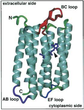 |
| FIGURE 1 Bacteriorhodopsin with its retinal chromophore (arrowhead). The extracellular (top) and the cytoplasmic side (bottom) of BR with their prominent loops and termini are indicated. This illustration of BR was calculated using the coordinates of Kimura et al. (1997) and the visualization program DINO (http://www.dino3d.org/). |
In this article, contact mode AFM is illustrated using membranes that contain the heptahelical protein bacteriorhodopsin (BR). This 26-kDa integral protein acts as a light-driven proton pump in Haloarchaea (Oesterhelt and Stoeckenius, 1973). Photoisomerization of the chromophore from all-trans to 13-cis retinal initiates the unidirectional translocation of one proton across the cell membrane (reviewed by Oesterhelt et al., 1992; Lanyi, 1997). This establishes an electrochemical proton gradient across the membrane that can then be used for ATP synthesis and other energy-requiring processes in the cell. BR forms trimers and highly ordered two-dimensional (2D) trigonal crystal lattices (parameters: a = b = 6.2nm, γ = 60°) in the native membrane of the bacterium Halobacterium salinarum, these crystalline patches are termed purple membrane because of their color (Blaurock and Stoeckenius, 1971). The flatness of these crystalline membrane patches makes them very suitable for AFM. Highresolution three-dimensional structures of BR (Fig. 1) have been determined by electron and X-ray diffraction (for a review, see Cartailler and Luecke, 2003). In BR, the prosthetic group retinal (see Fig. 1; arrowhead) is bound covalently by a protonated Schiff base to K216 of helix G of the protein (the seven transmembrane α helices are generally denoted A to G). With the AFM it is the protruding domains, i.e., the termini and connecting loops between the helices, that are visualized, not the helices themselves that are embedded in the lipid bilayer. On the cytoplasmic side, the major protrusions of BR are the loop connecting the transmembrane α helices A and B and that connecting E and F (AB and EF loops; Fig. 1), of which the EF loop appears to be highly flexible (Müller et al., 1995a). On the extracellular side the protruding B-C interhelical loop (BC loop; Fig. 1) forms a β hairpin and is fairly rigid.
The procedures described for BR in this article constitute a basis for sample preparation and application of AFM on other biological membranes.
A. Materials: Preparation of Mica Supports
Polished ferromagnetic stainless steel disks of 11mm diameter (manufactured by the internal workshop services of the Biozentrum, Basel, Switzerland)
Teflon sheets of 0.25 mm thickness (Maag Technic AG, Birsfelden, Switzerland)
Mica sheets with a thickness between 0.3 and 0.6 mm (Mica House, 2A Pretoria Street, Calcutta 700 071, India)
"Punch and die" set from Precision Brand Products Inc. (2250 Curtiss Street, Downers Grove, IL 60515)
Ethanol [purity: >96% (v/v)]
Loctite 406 superglue (KVT König, Dietikon, Switzerland)
Araldite Rapid: Two-component epoxy glue from Ciba-Geigy, Basel, Switzerland
Scotch tape (3M AG, Rüschlikon, Switzerland)
B. Materials: Bacteriorhodopsin and Buffers
Sodium azide (NAN3, Fluka Cat. No. 71289)
Tris [H2NC(CH2OH)3, Merck Cat. No. 1.08382.2500]
Magnesium chloride hexahydrate (MgCl2·6H2O, Fluka Cat. No. 63064)
Potassium chloride (KCl, Merck Cat. No. 1.04936.1000)
Purple membranes of H. salinarum (source: see Acknowledgments)
Stock suspension of purple membrane fragments: 0.25mg/ml in double-distilled water containing 0.01% NaN3 (stored at 4°C and protected from unnecessary light irradiation)
C. Instrumentation
A commercial multimode AFM equipped with a 120-µm scanner (j-scanner) and a liquid cell (Digital Instruments, Veeco Metrology Group, Santa Barbara, CA)
Oxide-sharpened Si3N4 micro cantilevers of 100 and 200 µm length, and nominal spring constants of 0.08 and 0.06N/m from Olympus Optical Co. Ltd., Tokyo, Japan, and from Digital Instruments, Veeco Metrology Group, respectively.
A. Preparation of Mica Supports for Sample Immobilization
Steps
- Punch Teflon disks of 0.5in. and mica disks of 0.25 in. diameter using the "punch and die" set and a hammer.
- Clean the steel and Teflon disks with ethanol and paper wipes.
- Glue a Teflon disk centrally on a steel disk using the Loctite 406 superglue and allow the glue to dry.
- Glue a mica disk centrally on the Teflon surface of the Teflon-steel disk with the Araldite twocomponent epoxy glue.
- Let the supports dry overnight.
B. Preparing Bacteriorhodopsin for AFM Imaging
Solutions
- Adsorption buffer: 20mM Tris-HCl (pH 7.8), 150mM KCl
- Imaging buffer for the extracellular side (ES-imaging buffer): 20mM Tris-HCl (pH 7.8), 150mM KCl, 25mM MgCl2
- Imaging buffer for the cytoplasmic side (CS-imaging buffer): 20mM Tris-HCl (pH 7.8), 150mM KCl
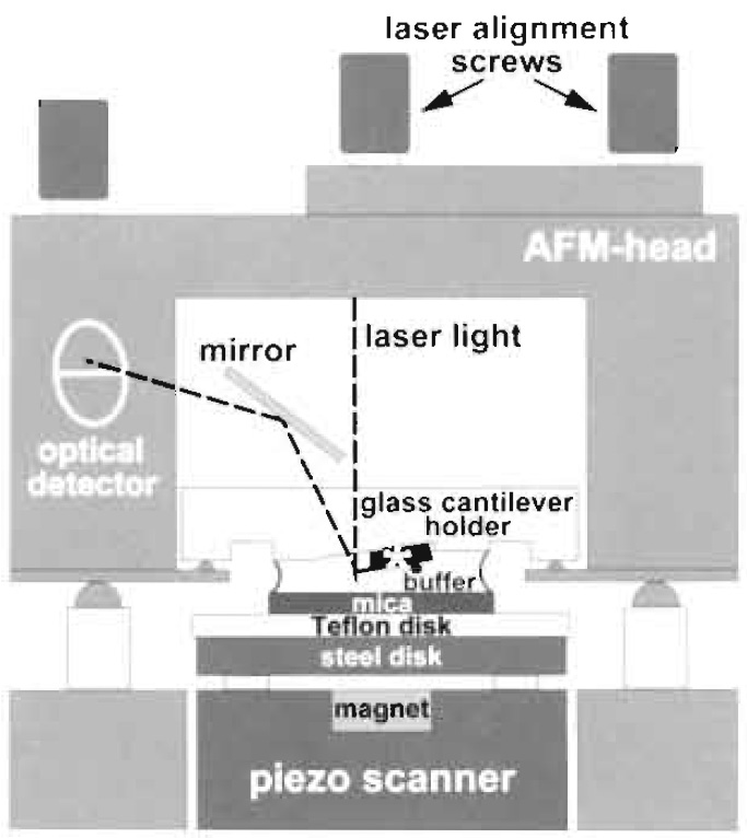 |
| FIGURE 2 Schematic diagram of the atomic force microscope setup for imaging in liquid. The piezo scanner moves the sample in xyz directions under the fixed cantilever (marked by an asterisk). |
- Dilute and mix 3µl of purple membrane stock solution with 30µl of adsorption buffer in an Eppendorf tube.
- Cleave the mica by applying Scotch tape to the upper surface and then peeling off until a new smooth intact mica surface is exposed. This new surface is clean and molecularly flat, suitable for deposition of the specimen to be imaged.
- Pipet 33µl of the diluted purple membranes on the hydrophilic surface of the freshly cleaved mica support.
- Allow the sample to adsorb for 15 to 30min.
- Wash away purple membrane fragments that are not firmly attached to the mica by removing approximately two-thirds of the fluid volume from the mica surface and readding the same volume of the desired imaging buffer. Repeat this washing procedure at least three times.
- Transport the specimen support and its associated fluid onto the piezo scanner of the AFM.
- Place the AFM head with its mounted fluid cell and cantilever on the scanner (see Fig. 2).
- Make sure that the space between the mica surface and the cantilever-fluid cell contains enough of the corresponding imaging buffer to avoid drying of the specimen during the imaging experiment. An experiment may last several hours.
- Align the laser spot onto the cantilever and the reflecting beam into the photodiode with the appropriate laser alignment screws. Caution: It is very important not to put any reflective objects into the laser trajectory in order to avoid reflection of the laser light into your eyes! Additionally, wear appropriate protection glasses!
C. Operation of the AFM
All measurements are carried out under ambient pressure and at room temperature.
These steps assume basic knowledge of AFM operation.
- Let the instrument equilibrate thermally.
- Set the scan size to zero to prevent specimen deformation and contamination of the tip after engagement.
- Initiate engagement process, i.e., permit the tip to approach the surface.
- As soon as the tip is engaged, and prior to scanning the surface, set the operating point of the instrument to forces below 100pN, i.e., minimal force.
- Calibrate the deflection sensitivity of the cantilever using the force calibration menu of the control computer.
- Start imaging and keep the forces during scanning as small as possible by correcting manually for thermal drift.
- Optimize the feedback parameters of the system, i.e., the integral gain and the proportional gain, by increasing their values. If the feedback loop starts to oscillate, introducing noise, reduce these gains until the noise goes away.
- Record two images of 512 by 512 pixels simultaneously at low magnification (frame size >1µm), one showing the height signal in the trace direction and the other the deflection signal in the retrace direction. Set the scan speed to two to four lines per second. Crystalline structures are usually recognized more easily in the deflection signal image than in the height image.
- Find and centre a suitable purple membrane fragment. Zoom in and set the scan speed to four to six lines per second. Record images of the height signals in both the trace and retrace directions at high magnification (frame size <1µm). Comparison of the trace and the retrace images allows deformation of the sample in the fast scan direction to be detected. Such deformations can be minimized by working at minimal force. At such high magnifications, the scan range of the z piezo can be reduced to avoid limitation of the axial z resolution that might otherwise occur because of rounding errors during (16-bit) digitalisation of the analogue signal (AD conversion).
IV. COMMENTS
The following sections explain and help understand the features observed on the topographies acquired during the AFM experiment.
Figure 3 shows a typical low-magnification topograph of purple membrane fragments adsorbed on mica. The diameter of the BR crystals varies between 0.5 and 1.5µm. The number of adsorbed membrane fragments depends on the adsorption buffer and time and on the concentration of the purple membrane suspension deposited on the mica. It is advantageous not to adsorb membranes too densely on the mica surface; this decreases the probability to contaminate the AFM tip. Two different surfaces can be discerned: The extracellular side of purple membrane is fairly flat (Fig. 3; arrows), whereas the cytoplasmic side is characterized by protruding bumps of 10-30nm in diameter (Fig. 3; arrowheads) (Müller et al., 1995b, 1996). A feature that can be used to differentiate further between the two sides is the small difference in thickness seen when scanning in CS-imaging buffer. Purple membranes exposing the cytoplasmic side appear slightly thinner than those exposing the extracellular side. As described by Müller and Engel (1997), pH and electrolyte concentration affect the apparent height measured between the mica and the cytoplasmic or the extracellular side of the purple membrane. This results from different surface charge densities.
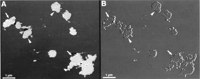 |
| FIGURE 3 AFM images of purple membrane at low magnification: height (A) and deflection (B) signals recorded in trace and retrace directions, respectively. Membrane patches exposing the cytoplasmic side (arrowheads), which are decorated by small debris, can be distinguished from patches exposing the flat extracellular side (arrows). The membrane patches have a height of ~6 nm when imaged in CS-imaging buffer. Vertical brightness ranges: 12nm (A) and 1nm (B). |
B. The Extracellular Surface of Purple Membrane
At high magnification, the appearance of the extracellular side of BR is characterized by protrusions extending 0.5 ± 0.1 nm out of the lipid bilayer (Fig. 4A and inset). The β hairpin in the loop connecting the transmembrane α helices B and C of BR constitutes the main portion of the observed protrusion.
The resolution of a micrograph containing a regular structure can be estimated from its power spectrum, i.e., its 2D Fourier transformation image. This was calculated from the topograph of the extracellular side of BR (Fig. 4A) and is displayed in Fig. 4B. Most software packages delivered with atomic force microscopes enable calculation of power spectra from recorded AFM topographs. Various public domain programs such as NIH image or ImageJ, both from the National Institutes of Health (Bethesda, MD), or SXM from the University of Liverpool (Liverpool, United Kingdom), have such algorithms implemented and can be downloaded for free (NIH image: http://rsb.info.nih.gov/ nih-image/; ImageJ: http://rsb.info.nih.gov/ij/; and SXM: http://reg.ssci.liv.ac.uk/).
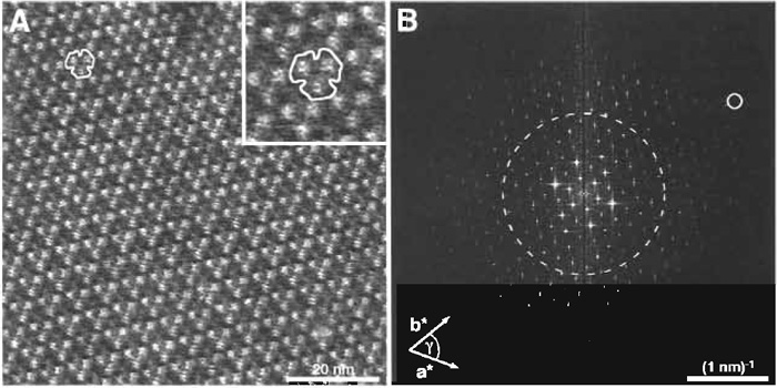 |
| FIGURE 4 (A) The extracellular side of purple membrane at high magnification. For clarity, the area around the contoured BR trimer was enlarged and is displayed in the inset (frame size: 17 × 17 nm). (B) Power spectrum calculated by Fourier analysis from the image in A. The (3, 10) diffraction spot (small circle) is marked and represents a resolution of 0.46 nm. The broken circle represents the 1-nm resolution limit. Vertical brightness range: 0.8 nm (A and inset in A). |
The larger the distance of the discernable spots from the origin in a power spectrum, the higher the resolution of the topograph. Here, spots extend beyond the 1-nm resolution limit (see broken circle in Fig. 4B). To calculate the resolution at a selected diffraction spot, Eq. (1) can be used. This equation is applicable to all lattice types, e.g., for trigonal, hexagonal, square, or orthorhombic lattices, which occur frequently in native and reconstituted 2D crystals of membrane proteins (for further reading on crystallography, see Misell and Brown, 1987).
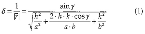 |
where δ is resolution; r- (r raised to bar) is vector from origin to the diffraction spot in Fourier space; a and b are basic lattice vectors in real space; γ is the angle between the basic lattice vectors; and h and k are Miller indices of the diffraction spot.
Example: The encircled spot (h, k) = (3, 10) in Fig. 4B corresponds to a lateral resolution of 0.46nm assuming the lattice parameters of BR (a = b = 6.2nm, γ = 60°).
 |
| FIGURE 5 Force-dependent topography of the cytoplasmic surface of a purple membrane. The area above the broken line was recorded at minimal force applied to the AFM stylus (≤100pN). At this force, the flexible EF loop is fully extended, whereas at a stylus force of ~200pN (area below the broken line) the loop is pushed away by the scanning tip and is therefore almost not visible anymore. For clarity, areas (frame size: 7 × 7nm) around the contoured trimers recorded at minimal force (broken circle; inset top left) and at a force of ~200 pN (solid circle; inset bottom left) are displayed enlarged as insets. Occasionally, defective BR trimers with a monomer missing can be found (arrowheads). Vertical brightness range: 1.2 nm. |
Imaging of the cytoplasmic surface of BR is force dependent because of the flexible EF loop (Müller et al., 1995a). At minimal force (≤100pN) applied by the AFM stylus (Fig. 5; area above the broken line and inset top left), the fully extended EF loops can be discerned as protrusions of 0.8 ± 0.2nm height. These become less prominent or even disappear if the loading force is increased to ~200pN (Fig. 5; area below the broken line and inset bottom left). At this force, the AB loops become visible with a height of 0.6 ± 0.1nm above the lipid bilayer. The advantage of such force-induced conformational changes is that shorter loops otherwise covered by the bigger ones can be visualized.
V. PITFALLS
A. Damping of Vibrations
For high-resolution AFM imaging, a vibrationally and acoustically isolated setup of the microscope is crucial. Antivibration and damping tables or lead platforms suspended by bungee cords offer excellent vibration damping. Acoustic isolation of the AFM can be achieved efficiently by installing a vacuum bell jar around the microscope.
B. Adjustment of Buffer for High-Resolution AFM Imaging
Topographs of this membrane protein with a lateral resolution of 0.41nm (Stahlberg et al., 2001) can be recorded reproducibly with the AFM, provided the imaging buffer is adjusted correctly (Müller et al., 1999) and the force applied to the tip is minimized. Under nonoptimal imaging conditions, even the smallest force that is adjustable by the instrument can be too high, leading to deformation of the biomolecules, e.g., concealing the EF-loop in BR (Fig. 5, lower portion). The effective interaction force acting between the AFM stylus and the specimen is determined by the force applied to the stylus, the electrostatic repulsion, and the van der Waals attraction between the two surfaces. By adjusting pH and ionic strength of the imaging buffer, van der Waals attraction and electrostatic repulsion between tip and sample can be balanced. The best imaging conditions are determined by recording and analyzing force-distance curves between tip and sample in different buffers. Conditions that yield force curves showing a small repulsion are ideal for highresolution imaging. Under these conditions the tip is assumed to surf on a cushion of electrostatic repulsion, thereby minimizing the deformation experienced by the biomolecules. This screening method revealed the two slightly different imaging buffers for BR mentioned earlier, i.e., CS- and ES-imaging buffer. For further reading on this topic, see Müller et al. (1999), where buffer conditions for different biological samples are discussed.
At this time, no commercial AFM tips are available with ideal point probes and perfect geometries in the subnanometer range. Therefore, tip effects and artefacts arising from the tip geometry are unavoidable and have to be considered when interpreting AFM topographies (for further reading on tip effects and artefacts, see Xu and Arnsdorf, 1994; Schwarz et al., 1994). Tip effects occur when the probe does not have a single, small, and sharp interaction area with the sample. This leads to an AFM image that represents a convolution of the sample features with the tip shape. To be sure of having acquired the correct surface structure and not an artefact, the same surface topography of the object being investigated has to be reproduced several times using different tips from different batches. Tip artefacts can also be identified by changing the direction in which the AFM tip scans the sample (scan angle), as artefacts will rotate correspondingly (Xu and Arnsdorf, 1994). Ordered structures, e.g., mosaic 2D crystals, that are differently oriented with respect to the scan direction of the AFM tip, are also good indicators for tip artefacts. Ideally, the building blocks of the crystal, e.g., the BR trimer, should look the same in the differently oriented crystals. Finally, structures of samples that have been determined by other methods, e.g., the structure of BR by electron and X-ray crystallography, can be used to further compare and confirm AFM data.
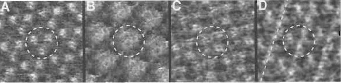 |
| FIGURE 6 Tip-induced effects and artefacts on the extracellular surface of bacteriorhodopsin. (A) Artefact- free and (B-D) artefacteous topographies of BR. In B the characteristic central depression at the threefold axis of the BR trimer is absent. The central trimer in C resembles a tetramer. In D the protrusions are not clearly separated, but connected along the broken line. In all images the central trimers are marked by broken circles. The frame sizes in A to D are 17 nm. The heights are 0.8 nm (A), 1.3 nm (B), 0.8 nm (C), and 0.8 nm (D). |
VI. CONCLUDING REMARKS
This article presented procedures for sample preparation and AFM imaging of native 2D crystals of bacteriorhodopsin. The experience gained will enable the readers to perform similar AFM experiments with other biological membranes.
This work was supported by the Swiss National Research Foundation, the M. E. Müller Foundation, the Swiss National Center of Competence in Research (NCCR) "Structural Biology," and the NCCR "Nanoscale Science." The authors are indebted to Dr. Ansgar Philippsen for Fig. 1 and to Professors Dieter Oesterhelt (Max-Planck-Institut fiir Biochemie, Martinsried, Germany) and Georg Büdt (Forschungszentrum Jülich, Jülich, Germany) for kindly providing us with BR. The authors acknowledge Dr. David Shotton for constructive comments on the manuscript.
References
Binnig, G., Quate, C. F., and Gerber, C. (1986). Atomic force microscope. Phys. Rev. Lett. 56, 930-933.
Blaurock, A. E., and Stoeckenius, W. (1971). Structure of the purple membrane. Nature New Biol. 233, 152-155.
Cartailler, J. P., and Luecke, H. (2003). X-ray crystallographic analysis of lipid-protein interactions in the bacteriorhodopsin purple membrane. Annu. Rev. Biophys. Biomol. Struct. 32, 285- 310.
Engel, A., Lyubchenko, Y., and M(iller, D. J. (1999). Atomic force microscopy: A powerful tool to observe biomolecules at work. Trends Cell Biol. 9, 77-80.
Engel, A., and Müller, D. J. (2000). Observing single biomolecules at work with the atomic force microscope. Nature Struct. Biol. 7, 715-718.
Fotiadis, D., Scheuring, S., Miiller, S. A., Engel, A., and Müller, D. J. (2002). Imaging and manipulation of biological structures with the AFM. Micron 33, 385-397.
Kimura, Y., Vassylyev, D. G., Miyazawa, A., Kidera, A., Matsushima, M., Mitsuoka, K., Murata, K., Hirai, T., and Fujiyoshi, Y. (1997). Surface of bacteriorhodopsin revealed by high-resolution electron crystallography. Nature 389, 206-211.
Lanyi, J. K. (1997). Mechanism of ion transport across membranes: Bacteriorhodopsin as a prototype for proton pumps. J. Biol. Chem. 272, 31209-31212.
Müller, D. J., Bfildt, G., and Engel, A. (1995a). Force-induced conformational change of bacteriorhodopsin. J. Mol. Biol. 249, 239-243.
Müller, D. J., and Engel, A. (1997). The height of biomolecules measured with the atomic force microscope depends on electrostatic interactions. Biophys. J. 73, 1633-1644.
Müller, D. J., Fotiadis, D., Scheuring, S., Müller, S. A., and Engel, A. (1999). Electrostatically balanced subnanometer imaging of biological specimens by atomic force microscope. Biophys. J. 76, 1101-1111.
Müller, D. J., Schabert, F. A., Büldt, G., and Engel, A. (1995b). Imaging purple membranes in aqueous solutions at subnanometer resolution by atomic force microscopy. Biophys. J. 68, 1681-1686.
Müller, D. J., Schoenenberger, C.-A., Bfildt, G., and Engel, A. (1996). Immunoatomic force microscopy of purple membrane. Biophys. J. 70, 1796-1802.
Oesterhelt, D., and Stoeckenius, W. (1973). Functions of a new photoreceptor membrane. Proc. Natt Acad. Sci. USA 70, 2853-2857.
J. Bioenerg. Biomembr. 24, 181-191.
Schwarz, U. D., Haefke, H., Reimann, P., and G/Jntherodt, H.-J. (1994). Tip artefacts in scanning force microscopy. J. Microsc. 173, 183-197.
Stahlberg, H., Fotiadis, D., Scheuring, S., R6migy, H., Braun, T., Mitsuoka, K., Fujiyoshi, Y., and Engel, A. (2001). Two-dimensional crystals: A powerful approach to assess structure, function and dynamics of membrane proteins. FEBS Lett. 504, 166-172.
Stolz, M., Stoffier, D., Aebi, U., and Goldsbury, C. (2000). Monitoring biomolecular interactions by time-lapse atomic force microscopy. J. Struct. Biol. 131, 171-180.
Xu, S., and Amsdorf, M. F. (1994). Calibration of the scanning (atomic) force microscope with gold particles.
J. Microsc. 173, 199-210.
Support our developers