The expected distribution of different phenotypic classes dealing with a quantitative trait can often be obtained using a binomial distribution. This is defined as a distribution having only two possible outcomes (e.g. dominant vs. recessive allele) each with a known probability. Although in an experiment like the ones described earlier in this section, the probabilities of dominant and recessive alleles are equal, in actual situation the distribution of dominant vs. recessive alleles may vary as in the negro populations in USA (dominant alleles = 70%; recessive alleles 30%; see Fig. 4.4). The most popular example of binomial distribution is tossing of a coin, with equal probability of head and tail i.e.
p(H)=
p(T)= 0.5. Similarly, in a dice having six faces the probability of success of getting six, is
p(S) = 1/6 and that of the failure is
p(F)= 5/6. In binomial distribution probability of success is represented as
p and that of failure is
q = (1 -
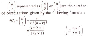
p). The popular form of binomial distribution is given as follows :


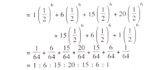
Utilizing the above formula for 3 gene pairs, the binomial distribution will be as follows
(p =
q = 0.5).


It should be noted that when
p =
q = 0.5, then the coefficients only determine the ratio, the denominator being the same. In such a case an easier method is Pascal's triangle given in Table 4.2.
However, if
p ≠
q, as in Figure 4.4
(p = .70 and
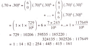
q = .30), then the distribution will differ. For three gene pairs the distribution will be as follows

From the above examples it is clear that a symmetric distribution is obtained, if
p =
q = 0.5, but the distribution becomes asymmetric, if
p ≠
q.

