Statistics

Statistical manipulation is often necessary to order, define, and/or organize raw data. A full analysis of statistics is beyond the scope of this work, but there are some standard analyses that anyone working in a cell biology laboratory should be aware of and know how to perform. After data are collected, they must be ordered, or grouped according to the information sought. Data are collected in these forms:



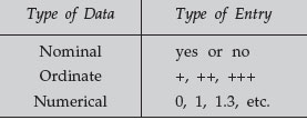
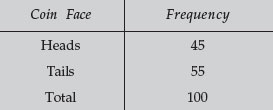
When collected, the data may appear to be a mere collection of numbers, with few apparent trends. It is first necessary to order those numbers. One method is to count the times a number falls within a range increment. For example, in tossing a coin, one would count the number of heads and tails (eliminating the possibility of it landing on its edge). Coin flipping is nominal data, and thus would only have 2 alternatives. If we flip the coin 100 times, we could count the number of times it lands on heads and the number of tails. We would thus accumulate data relative to the categories available. A simple table of the grouping would be known as a frequency distribution, for example:



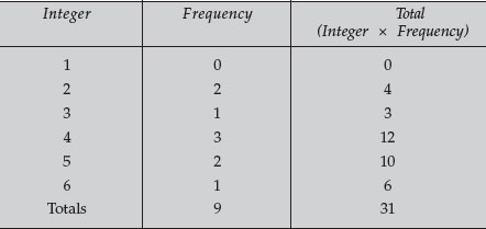
Similarly, if we examine the following numbers: 3, 5, 4, 2, 5, 6, 2, 4, 4, several things are apparent. First, the data need to be grouped, and the first task is to establish an increment for the categories. Let us group the data according to integers, with no rounding of decimals. We can construct a table that groups the data.



Mean, Median, and Mode
From the data, we can now define and compute 3 important statistical parameters

The mean is the average of all the values obtained. It is computed by the sum of all of the values (Σx) divided by the number of values (n). The sum of all numbers is 31, while there are 9 values; thus, the mean is 3.44.



The median is the midpoint in an arrangement of the categories by magnitude. Thus, the low for our data is 2, while the high is 6. The middle of this range is 4. The median is 4. It represents the middle of the possible range of categories.

The mode is the category that occurs with the highest frequency. For our data, the mode is 4, since it occurs more often than any other value. These values can now be used to characterize distribution patterns of data. For our coin flipping, the likelihood of a head or a tail is equal. Another way of saying this is that there is equal probability of obtaining a head or not obtaining a head with each flip of the coin. When the situation exists that there is equal probability for an event as for the opposite event, the data will be graphed as a binomial distribution, and a normal curve will result. If the coin is flipped 10 times, the probability of 1 head and 9 tails equals the probability of 9 heads and 1 tail. The probability of 2 heads and 8 tails equals the probability of 8 heads and 2 tails and so on. However, the probability of the latter (2 heads) is greater than the probability of the former (1 head). The most likely arrangement is 5 heads and 5 tails.

When random data are arranged and display a binomial distribution, a plot of frequency versus occurrence will result in a normal distribution curve. For an ideal set of data (i.e., no tricks, such as a 2-headed coin, or gum on the edge of the coin), the data will be distributed in a bell-shaped curve, where the median, mode, and mean are equal.

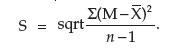
This does not provide an accurate indication of the deviation of the data, and in particular, does not inform us of the degree of dispersion of the data about the mean. The measure of the dispersion of data is known as the standard deviation. It is shown mathematically by the formula:



This value provides a measure of the variability of the data, and in particular, how it varies from an ideal set of data generated by a random binomial distribution. In other words, how different it is from an ideal normal distribution. The more variable the data, the higher the value of the standard deviation.

Other measures of variability are the range, the coefficient of variation (standard deviation divided by the mean and expressed as a percent) and the variance.

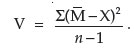
The variance is the deviation of several or all values from the mean and must be calculated relative to the total number of values. Variance can be calculated by the formula:



All of these calculated parameters are for a single set of data that conforms to a normal distribution. Unfortunately, biological data do not always conform in this way, and often sets of data must be compared. If the data do not fit a binomial distribution, often they fit a skewed plot known as a Poisson distribution. This distribution occurs when the probability of an event is so low that the probability of its not occurring approaches 1. While this is a significant statistical event in biology, details of the Poisson distribution are left to texts on biological statistics.

Likewise, one must properly handle comparisons of multiple sets of data. All statistics comparing multiple sets begin with the calculation of the parameters detailed here, and for each set of data. For example, the standard error of the mean (also known simply as the standard error) is often used to measure distinctions among populations. It is defined as the standard deviation of a distribution of means. Thus, the mean for each population is computed and the collection of means are then used to calculate the standard deviation of those means.

Once all of these parameters are calculated, the general aim of statistical analysis is to estimate the significance of the data, and in particular, the probability that the data represent effects of experimental treatment, or conversely, pure random distribution. Tests of significance will be more extensively discussed in other volumes.