Band Limit and Appropriate Sampling in Microscopy
A. What Is "Sampling?"
In microscope images obtained with the help of electronic devices (e.g., CCD camera) or in a scanning microscope system, data are usually obtained (sampled) at equidistant coordinates in object space. The distance between these measurement positions is usually denoted as the "sampling distance." Current technology samples on orthogonal coordinates (rectilinear sampling) with appropriate sampling distances along the in-plane coordinates X, Y and the axial coordinate Z (for three-dimensional imaging).
For a deeper understanding of how to choose these distances correctly, it is useful to assume the intensity distribution near the detector (translated back to sample coordinates) to be a continuous function (Fig. 1). The equidistant sampling coordinates, at which the values of the image function are recorded, are depicted as dashed lines in Fig. 1. The fact that pixels have a discrete physical size is not considered here to keep the discussion simple. This pixel-size effect is described by a convolution and can be considered as a multiplicative modification of the optical transfer function (Sheppard et al., 1995). In the considerations given in this article, noise resulting from photons and/or the detector system is neglected.
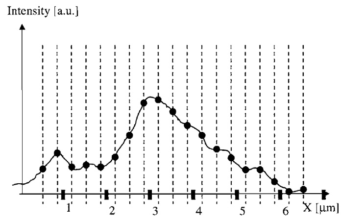 |
| FIGURE 1 Diagram of a microscope image as a continuous function over space (here indicated as the X coordinate). Dashed lines indicate the points at which the function is sampled (its value is recorded). |
Any physical function (e.g., as shown in Fig. 1) can be decomposed into a sum of sine waves, each with a different frequency, amplitude, and zero position (socalled phase). To exactly represent a function, this sum generally contains an infinite amount of components. Such decomposition is useful especially in optics, as images of (linear) optical systems have the interesting property of only transmitting sine waves of the sample up to a fixed limiting frequency. A periodic fluorescence distribution with a count of maxima per µm above this limit frequency will appear as a uniform constant in the image. Such systems are often called "band-limited" systems, as only a compact, limited band of frequencies (from zero to the maximal transmittable frequency) is transferred. How well a defined frequency is transferred is depicted in the "optical transfer function (OTF)" as outlined in Fig. 2 for inplane imaging in a fluorescence wide-field microscope. The "spatial frequency" given on the X axis of this graph denotes the number of maxima per meter for each sine wave. The sum of all sine waves yields the perfect image. The transfer strength of the OTF (Y axis) denotes how well a sample consisting of only one spatial frequency (one such sine wave) would be transferred to the detector.
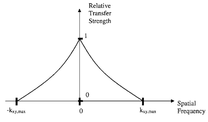 |
| FIGURE 2 The approximate shape of the in-plane optical transfer function of a fluorescence wide-field microscope. For spatial frequencies above the limiting frequency (kxy,max), no information can be transferred from the object to the microscope image. |
C. Band Limit of Optical Systems
1. Fluorescence Microscopy
When considering the sampling properties of microscopic imaging, a physical model (Young, 1985) of the microscope system has to be constructed. Due to the laws of physics, this OTF is zero beyond a welldefined limiting frequency (see Sheppard et al., 1994). In the case of wide-field fluorescence microscopy, the limiting frequency is as follows:
| kxy,max = | 2NA | , |
| λem |
with kxy,max denoting the maximal in-plane spatial frequency, λem the shortest detected vacuum wavelength of the fluorescence emission light, and NA = nsin(α) the numerical aperture defined by the refractive index n of the medium immersing the sample and the objective detecting light at an aperture half-angle of α.
Similarly, a limiting maximal transmittable axial spatial frequency kz,max can be given for sine waves with Z components as:
| kz,max = | NA | [1 - cos(α)] | . | |
| λem | sin(α) |
In confocal fluorescence microscopy, the illumination is confined to a diffraction-limited spot. At very small pinhole size, detection is also diffraction limited. A fluorophore needs to be excited and detected by the system, leading to a multiplicative process of excitation and detection. As a result, the aforementioned frequency limits have to be extended for the case of confocal fluorescence microscopy.
2. Aliasing
Because the images can be decomposed into the sine waves, it is useful to consider how an individual sine wave is sampled by the equidistant measurements. Figure 3 shows such a sine wave (solid black line) along with its values marked at equidistant sampling positions. Does such a measurement determine the frequency of the measured sine wave uniquely? As evident from Fig. 3 (dotted line), this is not the case, as multiple sine waves (these are called aliases) could possibly give the same measured values. However, if it is known that a maximal transmittable frequency exists, frequencies of sine waves in the image beyond that limit can be excluded as possible sources for this measurement. To guarantee a unique interpretation of a given measurement, all that needs to be done is to ensure all aliasing frequencies lie beyond the a priori known transmittable frequency limit.
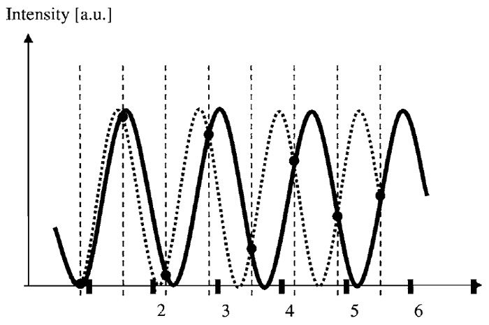 |
| FIGURE 3 Aliasing. Two sine waves with different spatial frequencies yield identical sampled values. A distinction based on the measured values is only possible when the dashed alternative wave can be excluded, as its frequency lies above the transfer limit. This gives rise to the Nyquist theorem stating that the maximal possible frequency in the image has to be sampled with more than two positions per wavelength. |
In an acquired image, multiple frequencies are measured simultaneously, and the aforementioned should be true for all spatial frequencies possibly present in the image. The highest frequencies in the image (just below the frequency limit, e.g., kimg < kmax = 5µm-1) turn out to be most critical, as their lowest frequency alias (kalias = ks - kimg, e.g., at ks = 11µm-1, kalias is 6µm-1) appears at lower frequencies than aliases of other lower frequency image contributions. If the image is sampled at least at twice its highest contained spatial frequency (ks > 2kimg), aliasing can be avoided, as interpretation of the sampled values is unique because kalias is above the limiting frequency kma x. In other words, the sampling frequency (ks = 1/D), as defined by the sampling distance D, has to exceed the maximal transmittable frequency by a factor of two (ks > kNq = 2kmax). This limiting sampling frequency kNq is called the Nyquist frequency.
II. INSTRUMENTATION
Selection of the appropriate sampling distances is crucial for almost all optical systems with computerized image acquisition. In the field of optical microscopy, one has to discriminate among fluorescence-, transmission-, and reflection-based systems.
III. PROCEDURES
In the procedures suggested here, equations are stated for different microscopy arrangements.
Many imaging systems do not allow for any direct control over the size of the detector bins. CCD camerabased systems and digitizing micrographs on a scanner fall in this category. To select the appropriate sampling distance:
- Obtain the pixel pitch (P) of your CCD camera from the manufacturer/supplier. The pixel pitch is the distance in X and Y directions between successive pixels. Usually this is in the range of 5 to 20 µm. When binning is used during image acquisition, the pixel pitch has to be multiplied with the binning factor (e.g., with 2 × 2 binning: multiply the pixel pitch by 2). When digitizing micrographs, a corresponding value is given by either the pixel-to-pixel distance after scanning or the resolution of the micrograph, whichever value is bigger. When a micrograph is scanned, care has to be taken to account for all magnification factors to finally obtain a pixel size corresponding to the image plane.
- Make a list of available objectives. Note magnification (e.g., 40 or 63×) and numerical aperture (e.g., 0.9 or 1.3) for each of them. These values are usually engraved on the side of the objectives. If any postmagnification system (e.g., Zeiss Optovar) is available on your microscope, multiply the objective magnification with the appropriate factor. The obtained total magnification is called M.
- Calculate the in-plane sampling distance (Dxy) as dictated by the detector pixel pitch in the object plane for each objective, dividing the pixel pitch by the magnification:
Dxy = P M
- Calculate the maximum sampling distance (dmax) in the object plane from the numerical aperture of the objective and the vacuum wavelength of light used for imaging:
Wide - field fluorescence : dxy,max = λem 4NAobj
Transmission or phase microscopy: dxy,max = λ 2(NAobj + NAcond)
In wide-field illumination microscopy systems, λem should be the shortest detected emission wavelength (e.g., FITC λem= 500nm); in transmission microscopy, the shortest transmitted wavelength should be used (e.g., blue at λ = 400nm). Note that the numerical aperture of the condensor (NAcond) contributes equally as the objective numerical aperture to the final resolution, although the contrast may suffer in transmission microscopy with a high condensor numerical aperture. Also note that the value NAcond is taken for a fully open condensor aperture; a closed condensor aperture enhances the contrast but reduces NAcond and thus the resolution. - Ensure that Dxy < dxy,max by selecting the appropriate objective and/or postmagnification optics from the list.
CCD Example
Let's say the pixel pitch of your camera is 7 µm and you are using no binning. The question is whether using a 100×, 1.3 NA oil (n = 1.516) immersion objective with the standard microscope tube lens (i.e., M = 100), the sampling distance in the focal plane corresponding to
| Dxy = | 7 µm | = 70nm |
| 100 |
| dxy,max = | 500 nm | ≈ 96.15 nm > 70 nm, |
| 4 · 1.3 |
B. Confocal Systems (in Plane)
Confocal microscopy usually allows for free control over the sampling distance in the object plane by selecting an appropriate magnification ("zoom") and image size in pixels. A notable exception to this is a Nipkov-type disc-scanning system employing a CCD camera. For such systems, the maximum sampling distances (dxy,max and dz,max) corresponding to a confocal system have to be selected, although the protocol for the CCD camera should be followed.
- Calculate the maximum sampling distance (Sheppard, 1989; Wilson, 1990; Sheppard et al., 1994) from the parameters of the objective (see CCD procedure for definitions):
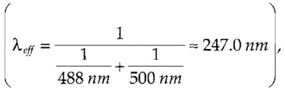
Confocal fluorescence (small pinhole): dxy,max = λeff , λeff = 1 4NAobj 1 + 1 λex λem
Confocal fluorescence (large pinhole): dxy,max = λeff 4NAobj
Confocal two-photon fluorescence (no pinhole): dxy,max = λex , 8NAobj
with λex being the irradiating wavelength (usually in the infrared).
Confocal reflection: dxy,max = λ 4NAobj
The strict theoretical limit even for large pinholes is the value given for small pinhole size. However, because the lateral high-frequency content for larger pinholes is negligible and usually lies well below the noise level, the "wide-field fluorescence" in-plane equation (as given earlier) can be applied, replacing the emission wavelength with the excitation wavelength. As a rule of thumb, consider pinhole sizes below 0.5 Airy discs in the pinhole plane as being small and sizes above 1.5 Airy discs as being large. In object space coordinates one Airy disc diameter (the first dark ring of a diffraction limited spot, assuming low NA) is
1.22 λem . NAobj
To compare with actual pinhole sizes, the pinhole has to be translated to the object space coordinates by the appropriate demagnification factor, if the pinhole size is not stated in Airy disc units in the microscope operating software. - For beam-scanning or object-scanning confocal systems, the in-plane sampling distance (Dxy) is usually stated somewhere on the screen. It can also be calculated from the image size in the object plane (Simg) and the number of pixels (Npix) along X or Y:
Dxy = Simg . Npix -1
This distance should be selected to be below the dxy, max calculated earlier.
Confocal Example
With the microscope parameters as stated in the wide-field example in Section III,A, confocal microscope illuminating at 488 nm
 |
with a small detection pinhole setting, would allow a maximum in-plane sampling distance of
| dxy,max ≈ | 247 nm | = 47.5 nm |
| 4·1.3 |
and the pixel-to-pixel spacing Dxy should be adjusted to a smaller value. For large pinholes, the following sampling distance should be acceptable:
| dxy,max = | 488 nm | ≈ 93.8 nm. |
| 4·1.3 |
C. Focus Series
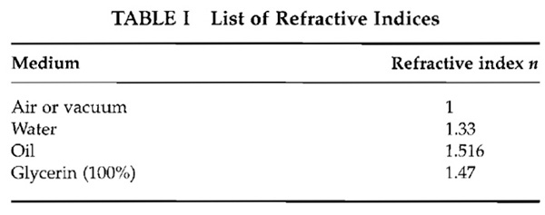
For the acquisition of focus series (Z stacks), an additional sampling limit along the axial direction also needs to be obeyed by choosing an appropriate distance between neighboring image planes. To calculate the corresponding maximum plane-to-plane distance (dz,max), the aperture half-angle of the objective (αobj) has to be known. Because this value is often not stated, it has to be calculated from the numerical aperture and the refractive index (n) of the immersion medium:
- Calculate the aperture half-angle of the objective as
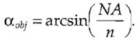
Approximate values for the refractive index are stated in Table I.
- Once the aperture half-angle is known, the maximum plane-to-plane distance is calculated as
Wide-field fluorescence: dz,max = λem sin(αobj) 2NAobj (1 - cos(αobj))
Transmission or phase microscopy: dz,max = λ sin(αmax) 2NAmax (1 - cos(αmax))
Confocal fluorescence: dz,max = λeff sin(αobj) , λeff = 1 2NAobj (1 - cos(αobj)) 1 + 1 λex λem
Confocal two-photon fluorescence: dz,max = λex sin(αobj) 4NAobj (1 - cos(αobj))'
with λex being the irradiating wavelength (usually in the infrared).
Reflection confocal: dz,max = λ 4n
For transmission or phase microscopy, NAmax and αmax denote the corresponding values of the greater of the condensor and objective numerical aperture. - Ensure that the distance between successive image planes (Dz) in object coordinates is belowdz,max.
Focus Series Examples
For the parameters of the wide-field fluorescence example just given, the appropriate spacing between successive image planes should be chosen to be below
| dz,max ≈ | 500 nm | sin(59°) | ≈ 339.6 nm | |
| 2·1.3 | (1- cos(59°)) |
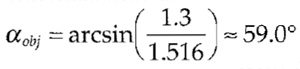
with the aperture half angle being estimated from the NA (1.3) and the refraction index of oil (n - 1.516) :
 |
Accordingly, the maximum spacing for confocal fluorescence microscopy (parameters as given in Section III,B) is calculated as
| dz,max ≈ | 247nm | sin(59°) | ≈ 167.8 nm | |
| 2·1.3 | (1- cos(59°)) |
IV. PITFALLS: CONTRAST AND SAMPLING
Suppose the object and its image consist of a sine wave with a single spatial frequency (e.g., 200nm distance between two maxima). The sampling limit requires sampling at more than the double frequency (i.e., Dxy < 100nm). If this image is sampled too close to the limiting frequency, there may be a problem. Depending on the exact position of the object, one may be fortunate enough to sample a maximum, then a minimum, a maximum again, and so on or, if unlucky, always sample half the maximum (see example in Fig. 4). In the latter case, the result would be indistinguishable from an object with zero frequency. Even when sampling at distances slightly below the required minimum distance, a very low contrast can result for images of small size. Therefore, one should oversample, such that at least one full period of the resulting envelope amplitude modulation is captured. In other words, with M pixels along a spatial direction, the stated maximum sampling distance should be lowered by multiplication with the factor M/(M + 1). For common image sizes (e.g., 512 x 512), this factor is negligible, but it can be substantial when acquiring only few Z sections (in which case M is the number of sections).
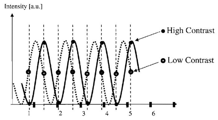 |
| FIGURE 4 For images containing only a few measured values, the measured contrast can be dependent on the exact phase of the sine wave to perform measurements even when the Nyquist limit frequency is obeyed (compare the contrast of closed and open circles). To ensure that at least one full variation of contrast is recorded, oversampling is recommended, as it leads to a required sampling frequency enhanced by a factor of (M + 1)/M with M measured sampled points. |
For some applications the sampling limit does not need to be obeyed. If, for example, the task is to count homogeneously filled cells with a fluorescent dye using a 20x, 0.9 NA objective, it makes a lot of sense to seriously undersample the data. For a cell to be identified it might suffice to detect two adjacent bright pixels. Thus the required sampling can, in some cases, depend on the size of the object structure to image. Undersampling (e.g., by binning) can reduce the amount of acquired data (important in screening applications), reduce the readout noise, dark current, and sometimes enlarge the field of view. In the mentioned application the introduced aliasing effects should be tolerable.
In other applications (e.g., neuronal imaging of dendrites) it may be very tempting to undersample the data. However, thin structures (such as dendrites) may occasionally be lost in some pixels because they happen to lie between two sample points. Such missing gaps can then render a computer-based analysis difficult, as the structures appear ruptured and will also cause serious problems when successive computerized deconvolution is applied to data. In these cases it can even be better to reduce the numerical aperture of the objective than to seriously undersample at high NA.
For some gray value-based image processing tasks, oversampling is recommendable (Young, 1996, 1988; Verbeek, 1985; Verbeek and vanVliet, 1993); e.g., if the aim is the precise determination of object positions, one should oversample data by a factor of at least 1.5 (sample at a 1.5 times smaller pixel pitch as compared to the limits given earlier). Simulations revealed (Heintzmann, 1999) that determination of the center of mass can result in a significant systematical error even when sampled according to the stated sampling limits. Furthermore, a smaller sampling distance determines more precisely where each photon hits the detector, thus leading to a slightly more precise estimate of the particle position (Heintzmann, 1999). Oversampling can also be useful when successive deconvolution of data is planned (see below). Note that with oversampling, the photon dose delivered to the sample can still be kept constant. Acquired images may look inferior at a first glance, but they still contain all the necessary information. Such data always allow for successive binning, resampling, and/or smoothing to enhance the visual appearance.
When the computerized deconvolution is applied to data, it is often useful to oversample data during data acquisition. The reason is that constrained deconvolution is capable of "guessing" high-frequency components in the object structure that have not been acquired. This is enabled by the use of prior knowledge about the object, e.g., its positivity or smoothness (Sementilli et al., 1993). In principle, acquired data can be resampled, but this always involves loss of information about the photon statistics, or even interpolation errors can result. Although software might be able to reconstruct on a denser grid than raw data, there may be (depending on the algorithm) some resampling involved, which in turn can skew the statistics of the deconvolution procedure, thus leading to inferior results. As a rule of thumb, a two-fold oversampling (two times smaller sampling distances as compared to the given limits) should suffice even for advanced deconvolution software.
Appendix: Derivation of Cut-Off Frequencies
To obtain the equations given in the text, an expression for the cut-off spatial frequency was derived and the Nyquist theorem applied, calculating the maximum sampling distance as half the distance corresponding to this cut-off spatial frequency. Note that this derivation is valid for high NA vector theory.
Electric field components of a plane wave can be described by a single point in Fourier space. Its distance to the origin is proportional to the inverse wavelength. A lens forms its image by the constructive interference of converging parallel beams. It can thus be described by a "cap" (Gustafsson et al. 1995) in Fourier space (Fig. 5a).
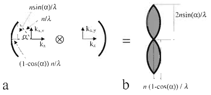 |
| FIGURE 5 Derivation of the region of support of the fluorescence wide-field optical transfer function (b) from an autocorrelation of interfering plane waves (a), all depicted in Fourier space. |
For incoherent fluorescence wide-field imaging, the intensity in focus describing the point spread function (PSF) is obtained as the square of the absolute magnitude of the electric field distribution. Because the optical transfer function (OTF) is the Fourier transformation of the PSF, it can be obtained as an autocorrelation of Fig. 5a, which is identical to the convolution with itself mirrored at the origin in Fourier space. The resulting region of support is depicted in Fig. 5b. The corresponding distances are the reciprocal values, which have to be halved, yielding the respective maximum sampling distance in XY and Z directions.
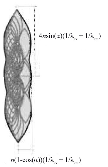 |
| FIGURE 6 Support of the optical transfer function for a confocal fluorescence microscope obtained by autocorrelation of Fig. 5b. |
In the case of confocal microscopy, photons have to be excited and detected. This leads to a multiplication of the probabilities of excitation PSF (corresponding to the OTF in Fig. 5b, but for λex) and the emission PSF (corresponding to the OTF in Fig. 5b). In Fourier space, this translates to a convolution of Fig. 5b as depicted in Fig. 6, yielding the appropriate equations for the confocal closed pinhole case. The size and shape of the pinhole is described by a multiplicative modification of the detection OTF with the Fourier transformed pinhole. The two-photon (no detector pinhole) derivation follows in a similar fashion, as its PSF is the square of the excitation PSF, which can be described by autocorrelation of Fig. 5b for λex.
The equation for confocal reflection microscopy is obtained by considering the possible scattering vectors when illuminating and detecting through the same objective (Fig. 7b).
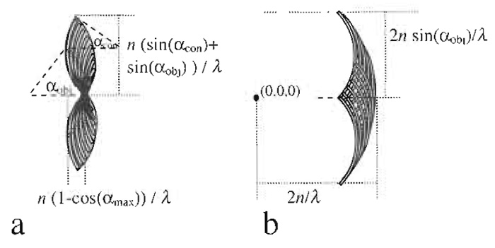 |
| FIGURE 1 Shape of object frequencies (scattering vectors) that can possibly be imaged with an incoherent wide-field transmission microscope (a) and a confocal reflection microscope (b). |
Acknowledgment
B. Rieger, S. H6ppner, E. Lemke, I. T. Young, and T. M. Jovin are thanked for their help in revising this manuscript and C. J. R. Sheppard for fruitful discussions on sampling.
References
Gustafsson, M. G. L., Agard, D. A., and Sedat, J. W. (1995). Sevenfold improvement of axial resolution in 3D widefield microscopy using two objective lenses. Proc. SPIE 2412, 147-156.
Heintzmann, R. (1999). "Resolution Improvement of Biological Light Microscopic, data." Ph.D. thesis, Institute of Applied Physics, University of Heidelberg, Germany.
Sheppard, C. J. R. (1989). Axial resolution in confocal fluorescence microscopy. J. Microsc. 154, 237-241.
Sheppard, C. J. R., Gu, M., Kawata Y., and Kawata, S. (1994). Threedimensional transfer functions for high-aperture systems. J. Opt. Soc. Am. A 11, 593-598.
Sheppard, C. J. R., Gan, X., Gu, M., and Roy, M. (1995). Signal-tonoise in confocal microscopes. In "'Handbook of Biological Confocal Microscopy" (J. B. Pawley, ed.), pp. 363-371. Plenum Press, New York.
Verbeek, P. W. (1985). A class of sampling-error free measures in oversampled band-limited images. Pattern Recogn. Lett. 3, 287-292.
Verbeek, P. W., and van Vliet, L. J. (1993). Estimators of 2D edge length and position, 3D surface area and position in sampled grey-valued images. Biolmaging 1, 47-61.
Young, I. T. (1985). Estimation of sampling errors. Cytometry 6, 273-274.
Young, I. T. (1988). Sampling density and quantitative microscopy. Anal. Quant. Cytol. Histol. 10, 269-275.
Young, I. T. (1996). Quantitative microscopy. IEEE Engineer. Med. Biol. Mag. 15, 59-66.
Support our developers