Three-Dimensional, Quantitative in vitro Assays of Wound Healing Behavior
Wound healing in vivo is a dynamic process involving the coordinated regulation of cell proliferation, cell migration, cell traction, and apoptosis (Clark, 1996). For instance, during dermal wound healing, inflammatory cells are induced to infiltrate a wound site primarily by factors released from platelets. Fibroblasts are stimulated to migrate up a chemotactic gradient of soluble factors, and possibly a haptotactic gradient of matrix-bound factors, released by the inflammatory cells and platelets into a provisional matrix composed primarily of fibrin and fibronectin. These fibroblasts proliferate and secrete collagen and other extracellular matrix molecules to form granulation tissue. The cells often contract this granulation tissue while continuing to secrete collagen. Ultimately, the cells die through apoptosis and leave a dense, collagenous, acellular scar as a reparative patch. The progression of fibroblast behavior is dictated in part by cues from the wound healing environment, such as soluble growth factors, integrin binding to network proteins, and mechanical stress associated with wound contraction. Therefore, it becomes a great challenge to design and implement bioassays that capture quantitatively the key features of wound healing in a controlled, but physiologically relevant manner. This article describes several assays that allow quantitative evaluation of fundamental aspects of cell behavior involved in the wound healing response-cell migration, chemotaxis, cell traction, and cell proliferation--in controlled environments with improved physiological relevance. The relevance of the assays is improved by examining cellular phenomena within three-dimensional (3D) hydrogels of biopolymers involved in wound healing, namely type I collagen and fibrin. Many studies have demonstrated dramatic differences in tissue cell behavior when cultured in a 3D gel rather than on a 2D substrate (Bell et al., 1979; Nusgens et al., 1984).
Trypsin (Product No. T6763), paraformaldehyde (Product No. 158127), ethylenediaminetetraacetic acid (EDTA) (Product No. E26282), CaCl2 (Product No. 21075), NaOH (Product No. 72079), bovine fibrinogen (Product No. 46312), bovine thrombin (Product No. T4265), and agarose (Product No. A2790) are from Sigma Chemical Company (St. Louis, MO). Vitrogen 100 bovine type I collagen (Product No. FXP-019) is from Cohesion Technologies, Inc. (Palo Alto, CA). Tissue culture medium, penicillin/streptomycin (pen-strep; Cat. No. 15070063, fungizone (Cat. No. 15240062), HEPES buffer (Cat. No. 15630080), phosphate- buffered saline (PBS; Cat. No. 10010023), and L-glutamine (Cat. No. 21051024) are from GIBCO Laboratories (Grand Island, NY). Fetal bovine serum (FBS; Product No. SH30073.02) is from HyClone Laboratories (Logan, UT). Polystyrene beads (Product No. 64130) are from Polysciences, Inc. (Warrington, PA). Stock Teflon (Product No. B-ZRT-2), stock polycarbonate (Product No. B-211040), and stock hydrophilic porous polyethylene disk (Product No. B-PEH-060/50) are from Small Parts (Miami Lakes, FL).
III. EQUIPMENT
Inverted microscope with computer-controlled stage and on-stage incubation system, biological hood, air or CO2 incubator.
A. Biopolymer Gel Solution Preparations
Type I Collagen Gel (2.0mg/ml)
Collagen gels are prepared by neutralizing stock type I collagen solution and raising the temperature to facilitate self-assembly of monomeric collagen into fibrils and forming an entangled network of fibrils with interstitial medium (Knapp et al., 1997).
Steps
- To make 1 ml of collagen, add the following reagents to a 15-ml conical tube in order in a biological safety cabinet/laminar flow hood under sterile conditions: 20 µl 1 M HEPES buffer, 132 µl 0.1 N NaOH, 100 µl 10 X MEM, 60 µl FBS, 1 µl pen/strep, 10 µl L-glutamine, and 677 µl Vitrogen 100.
- Mix gently by pipetting.
- Keep the solution on ice until ready to prepare the assay.
Note: The final solution should be a light pink color/red color indicating neutral pH.
B. Fibrin Gels (3.3 mg/ml)
Fibrin gels are prepared by enzymatically cleaving fibrinogen with thrombin in the presence of Ca2+ ions (Knapp et al., 1999).
- Fibrinogen solution A: Dissolve fibrinogen powder in a 20mM HEPES-buffered saline solution to a concentration of 30mg/ml. Pass the solution through a 0.20-µm filter. Store in 1-ml aliquots at -80°C.
- Thrombin solution B: Dissolve thrombin (250 units) in 1 ml sterile water and 9ml of PBS. Pass the solution through a 0.20-µm filter. Store in 100-µl aliquots at -80°C.
Gel Preparation
- Add 1 aliquot of fibrinogen solution A to 5ml 20mM HEPES-buffered saline to make a 5-mg/ml fibrinogen solution.
- In a separate vessel, add one aliquot of thrombin solution B to 1 ml unsupplemented M-199 no serum and 15µl of 2M CaCl2 solution to make solution C.
- Prepare cell suspension D in cell culture medium with the cell concentration six time the desired final concentration. Solution D will be diluted 1:6.
- Keep the solutions separated and on ice until you are ready to prepare the assay.
- To make the fibrin gel, mix one part of thrombin/ Ca2+ solution C, one part of cell suspension D, and four parts of fibrinogen solution A. Mix gently by pipetting and fill the assay chamber quickly.
Frequently, mixing of fibrin and collagen solutions generates many bubbles, which can affect the geometry and rheology of gels and blur microscopy images. To limit bubbles, apply a vacuum to conical tubes holding the solutions (for collagen, degas the solution after mixing but before gelation, for fibrin, degas the fibrinogen solution, thrombin solution, and cell culture medium before mixing) to draw dissolved air out of solution and into the vacuum. Make sure that the solution is not too close to the top of the conical tube (10ml or less).
Because the fibrin gel can form quickly, add the fibrinogen solution last and pipette the mixed solution into the assay chamber quickly.
Disrupting forming gels can affect structural and rheological properties that are important for cell behavior assays. Take care when handling the gels during and after formation.
The following assays were developed to examine phenomena associated with dermal wound healing and therefore incorporate dermal fibroblasts as the cell of choice. However, the assays can be adapted easily for other cell types (e.g., smooth muscle cells or corneal fibroblasts.) The key is to maintain tight control over cell populations and the cell density used in the assays, as cell behavior can vary widely from passage to passage, and cell density dramatically affects the potential for cell-cell signaling, which, if not accounted for, can cloud results. Cell densities delineated below are recommended but should be optimized according to the cell type and the phenomena to be studied.
V. CHEMOTAXIS ASSAY
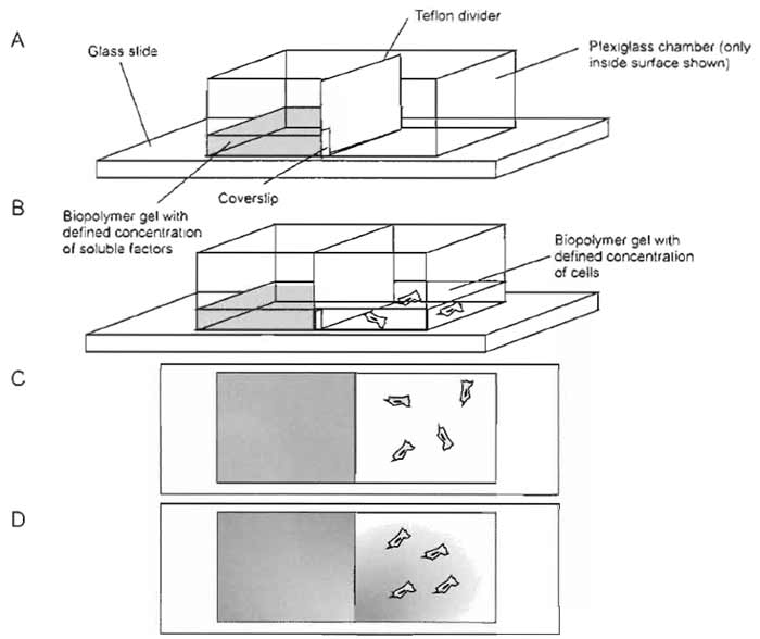
Chemotaxis experiments are performed in a conjoined 3D gel system (Knapp et al., 1999; Moghe et al., 1995). Manufacture of chemotaxis chambers and image analysis are involved. The experiments require machining of chemotaxis chambers (see later). The chambers allow the generation of a gradient of a protein/growth factor-sized diffusible species (Fig. 1). Briefly, one-half of the chamber is filled with collagen or fibrin solution and a defined concentration of chemotactic species, and the other, initially separated by a thin divider, is filled with an equal volume of biopolymer solution with a defined density of cells of interest. After removing the divider, a gradient of the species is formed in the gel with cells.
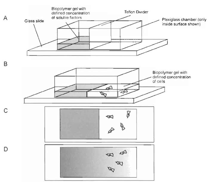 |
| FIGURE 1 Schematic of linear chemotaxis chamber preparation. The chamber consists of a hollow, plexiglass box that is sealed to a standard glass slide with vacuum grease. A Teflon plate divides the chamber into two sections. (A) One side of the chamber is filled with biopolymer gel with a defined concentration of chemotactic factor. For collagen assays, the chamber is placed in the incubator, and the biopolymer solution is allowed to gel. (B) The Teflon divider is removed, and the other half of the chamber is filled with biopolymer solution with a defined cell concentration. The chamber is returned to the incubator to facilitate gelation. (C) Initially, all of the chemotactic factor is in the left half of the chamber, and the cells in the right half are oriented randomly. (D) Over time, the soluble factor diffuses into the right half, and the cells (if responsive to the soluble factor) reorient and migrate in the direction of the gradient. |
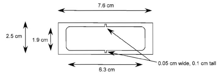 |
| FIGURE 2 Mechanical drawing of linear chemotaxis chamber. The chamber is machined from plexiglass (polycarbonate) and is 1.3cm high. A Teflon plate (1.2 × 0.05 × 2cm) is also required to fit into the notched area and divide the chamber in half. |
- Have chemotaxis chambers (at least 6-10) machined according to Fig. 2.
- Chambers are designed to fit on top of a standard microscope slide (7.5 × 2.5cm).
- Chambers have a groove at the midline for a thin, Teflon divider.
- Thoroughly clean chambers with soapy water and autoclave prior to each use
- Sterilize all chambers and glass slides.
- Under sterile conditions, secure bottom of chamber to glass slide with vacuum grease.
- Place Teflon dividers into grooves.
- Prepare solutions for assay (either fibrin or collagen).
- Each chamber requires ~3.5 ml biopolymer solution, which should be divided into two equal volumes of 1.75 ml/chamber.
- Add enough chemotactic factor to one of the volumes of the solution to generate the desired final concentration. Generally for growth factors, the working range is 0.1-100 ng/ml. This is now called "solution A."
- Add cells to the other half of the solution to a final concentration of 10,000 cells/ml. This is now called "solution B."
- Add 1.75ml of solution A to one-half of each chamber. This should fill the half approximately 3 mm.
- Secure another glass slide to the top of each chamber and place the chambers in a humidified incubator until gelation/self-assembly is complete.
- After gelation, remove chambers from the incubator and, again under sterile conditions, remove the Teflon divider.
- Mix solution B by pipetting to ensure uniform distribution of cells and fill the empty half of the chamber with 1.75 ml of solution B.
- Replace top glass slide, ensuring a good seal, and place back in humidified incubator for 24-36 h
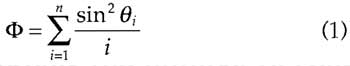
- At desired time points (typically 12-36h after gelation), place chamber under microscope and capture images of all cells through the thickness of the gel. This should be done with sufficient objective power (4× or greater) to observe the orientation of cells. This is facilitated greatly using automated microscopy/confocal microscopy with a motorized stage to build a mosaic, but can be done by hand if necessary. With automation, a projection mosaic of the gel containing cells is generated incorporating all planes throughout the thickness of the gel.
- For each cell, using standard image analysis packages (such as NIH Image), draw a line segment representing the prevailing orientation of the cell (Fig. 3) and calculate and record the angle, 0 (from 0° to 90° the line segment makes with the horizontal axis, which represents the direction of the chemotactic gradient.
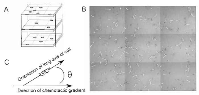
- For each cell, calculate sin2(θ)
- Determine the average value of sin2(θ) for all of the cells in a given chamber. In other words,
where n represents the number of cells (Fig. 3).
In the case of no chemotactic factor, cells should be oriented randomly. Therefore, the average angle should be 45° and Φ = 0.5. For a pure chemotactic response, θ = 0° and 9 = 0. Generally, values of Φ < 0.5 signify a chemotactic response, but results should be analyzed statistically after measuring the response in multiple chambers.
 |
| FIGURE 3 Chemotaxis analysis. (A) After a period of time (or at regular intervals, if desired), a composite, mosaic image of the cell-populated half of the chamber is captured and projected into one image. (B) The orientation of each cell is defined by tracing the long axis of the cell with a line. (C) The orientation of each line is compared to the orientation of the gradient via the angle θ. The response of the population is then evaluated using Eq. (1). |
- Control experiments should include no chemotactic factor, as well as uniform chemotactic factor (half-loading in both solution A and solution B).
- If imaging requires a large block of time, gels can be fixed with 2-4% paraformaldehyde to ensure equal exposure times to chemotactic gradients across experiments.
- To avoid settling of cells to the bottom of the gel due to gravity, prewarm solution B to ~28-30°C prior to filling the second half of the chamber. This is more crucial for experiments with collagen.
- Alignment of cells in the direction of the gradient may indicate a negative chemotaxis response. If the polarity of the cells cannot be determined easily, it is necessary to record the migration of the cells to confirm that they migrate toward the source of the factor (positive chemotaxis or chemoattraction) or away from the source (negative chemotaxis or chemorepulsion).
- Machine chambers identical to those described earlier, but add a small notch to the Teflon divider.
- When preparing the chamber, include a glass coverslip alongside the Teflon divider.
- Fill one-half of the chamber with biopolymer solution with a defined concentration of the peptide sequence and allow to gel.
- Fill the other half with biopolymer solution with defined cell concentration and allow to gel.
- Remove coverslip, but leave notched Teflon divider in place. This should create radial gradients (see Fig. 4).
- Transfer to microscope and quantify as described previously, with the exception that the direction of the gradient is now radially outward from the notch.
 |
| FIGURE 4 Schematic of radial chemotaxis assay for small chemotactic molecules. The assay is similar to the linear chambers, except that the Teflon divider remains in the chamber and has a small notch to restrict diffusion between the two halves. A glass coverslip prevents premature diffusion. |
Simple cell traction assays can be performed with either mechanically constrained, stressed gels or unconstrained, unstressed gels in various geometries (Neidert et al., 2002; Ehrlich and Rajaratnam, 1990). This section describes the simplest one to implement - cylindrical disks (Neidert et al., 2002; Tuan et al., 1994). The geometry is a hemisphere initially, but evolves to a cylindrical disk shape as the cell traction proceeds.
- With a sterile scribe, score a 1-cm-diameter circle in each well of a six-well plate.
- Prepare collagen or fibrin solution with a final cell concentration between 10,000 and 500,000 cells/ml.
- Carefully pipette 0.5ml collagen or fibrin solution into the scored region. The scratch in the culture plate should force the solution to maintain shape.
- Carefully place the plate in an incubator and allow solution to gel.
- After gelation, fill each well with 2.5 ml of culture medium with defined concentrations of the desired soluble factors.
- If the assay is for unstressed gels, with a sterile, flat spatula, gently pry the gels off of the bottom surface so that they are "free floating."
- Transfer the plate to a microscope and measure the thickness of the gel. When using a microscope equipped with motorized focus, this is done most easily by focusing on the top of the gel, recording the motor position, and then focusing on the bottom of the gel and determining the change in motor position, and therefore the thickness. For unstressed gels, also measure the diameter of the gel. (The diameter should remain unchanged for stressed gels.)
- Return the gels to the incubator.
- Repeat measurement performed in step 7 at regular intervals of your discretion. Once every 1-2 h is generally sufficient for a short duration (12-24h experiment. Once every 4-6h is sufficient for longer duration experiments. Return the samples to the incubator immediately after recording the thickness.
- After completion, normalize results by the original dimension and plot percentage compaction vs time for the various conditions.
- Gel thickness measurements reflect the gel rheology (and possibly cell proliferation) as much as cell traction. An intrinsic measure of the latter can be obtained by analyzing data using a mechanical model for cell-matrix interactions (Barocas et al., 1995; Barocas and Tranquillo, 1997a,b).
- If only measurements are desired for the constrained case, the sample can be attached to a force transducer (Eastwood et al., 1996; Kolodney and Wysolmerski, 1992).
- Cell alignment that typically results during the contraction of mechanically constrained gels can complicate the interpretation of data (Barocas and Tranquillo, 1997a,b).
Time-lapse cell migration assays in a 3D matrix can be performed to evaluate cell migration in two or three dimensions (Knapp et al., 2000; Shreiber et al., 2001, 2003). Both techniques require an automated image analysis system and an XY motorized stage. Motorized focus is advantageous for evaluation in 2D and is required for 3D.
Generally, it is advised to perform each experimental condition in triplicate. For instance, if the assay was to determine the effects of PDGF-BB on fibroblast migration and the experiment called for testing cells in the presence of 0, 10, 20, and 50ng/ml, then 12 wells would be needed.
The migration assay can be performed in practically any assay chamber. It is written here for a 96-well plate arrangement.
In these assays, data are recorded to fit to the persistent random walk model of cell migration (Dunn and Brown, 1987). This model implies that cell migration is purely random over long periods of time, but can have persistent direction over short period of times. To assess cell migration, there are three parameters, two of which are independent: persistence time, P; cell speed, S; and cell motility, bt. These three parameters are related via calculation of the mean-squared displacement (MSD) of the cells:
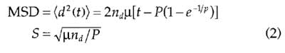 |
where nd= number of dimensions tracked (two for X-Y tracking, three for X-Y-Z tracking).
Both 2D and 3D analyses require complex image analysis codes that can perform object identification and/or correlation. Many software packages now include such algorithms, and they can also be programmed by the individual laboratories. The actual codes will differ according to the software packages, and presentation of a code is beyond the scope of this article. A brief outline for 2D and 3D is presented.
- Prepare collagen or fibrin solution with a final cell concentration between 7500 and 30,000 cells/ml and 5000-10,000 10-µm polystyrene after beads/ml. Beads serve as fiduciary markers to allow measurement of any drift in the stage or movement of the gel. They are especially crucial for 3D, high-magnification tracking and analysis.
- Pipette 100ml of collagen or fibrin solution into a well of the 96-well plate. Fill as many wells as warranted to complete the experimental test matrix.
- Carefully place the plate in an incubator and allow solution to gel.
- After gelation, fill each well with 100ml of cell culture medium with twice the defined concentration of the desired soluble factor(s) to yield the correct final concentration.
- Transfer the plate to an inverted microscope that includes an automated image analysis system and motorized stage, potentially motorized focus, and an environmental chamber to maintain proper humidity and CO2 concentration. Air-buffered media can be used (e.g., M199) if on-stage CO2 regulation is unavailable.
- Using a 10× objective, select a focal plane that is consistent among all of the wells.
- Move the stage from desired well to well and record images of each well. Build a mosaic image if necessary. Develop a numbering scheme to save the images (e.g., [date]_[condition]_[sample]_[image number]). Be sure to record the centroid position of each well so that the computer can move the microscope stage to those same positions at future time points.
- Determine the total duration of an individual interval, and the total number of intervals, which define the overall length of the time-lapse experiment. Be certain that your system is capable of capturing the desired number of images required for one complete interval in the time allocated. Generally, intervals should be as short as possible, so it frequently helps to work backward and determine how quickly the desired number of images can be captured. In this case, be sure to include a safety factor (usually a minute or two is sufficient to ensure that all required images are captured).
- Instruct the computer to return to each position, in sequence, record an image(s) of the well, move to the next position, etc. After the last picture in one interval has been recorded, the computer should instruct the stage to wait until the beginning of the next time interval to return to the first well. For instance, if a time interval is 10 min and all pictures from an interval are captured in 8 min, the computer should wait 2min to begin the next interval instead of immediately beginning the next time interval. Maintaining a consistent time interval simplifies data analysis greatly.
- Object identification can be performed during an experiment or off-line. In either case, the general scheme is the same: (a) capture image and (b) filter image to accentuate "objects," i.e., cells and beads.
Filtering usually involves- Equalizing contrast.
- Low-pass filter.
- Edge detection filter (e.g., Sobel).
- Generating a binary image based on an appropriate gray-scale level.
- Rejecting objects that are too big and/or too small.
- Recording the centroid position of objects, and correlating those positions, and possible shapes to the previous interval to track individual cells properly. Shape matching is not necessarily advised for tracking cells, as they change morphology during migration, but will certainly work for beads.
- Tabulate the cell/bead positions in a text file in a rational sequence. Include a flag to represent whether the object is a bead (1) or a cell (0). For instance.
Interval 1, Well 1, Object (cell or bead) 1, Type of object (Cell = 0, Bead = 1), Xposition 1, Yposition 1
Interval 1, Well 1, Object 2, Type, Xposition 1, Yposition 1 . . .
Interval 1, Well 2, Object 1, Type, X1, Y1
Interval 1, Well 2, Object 2, Type X1, Y1 ...
Interval 2, Well 1, Object 1, Type X2, Y2
Interval 2, Well 1, Object 2, Type X2, Y2...
Proceed to step 10.
Use the following steps for analysis of migration in 3D (must have automated focus). - Use the lowest power objective that generally allows you to focus on any object so that it is the only object in the volumetric field of view (FOV). To do this:
- Scan through the sample until you find an object.
- Maneuver the stage so that the object is in the center of the FOV and in focus.
- Make sure that the object is the only one in the volume immediately surrounding that object in all directions (including the focal plane, Z).
- Recenter and focus the object and record the position of the stage and focus on the computer
- Select the cells and beads to track. Optimally, search for a bead with many (at least three to four; the more the better) cells within 200-400µm of the bead, but not within the FOV. The motion of that bead would then represent the local absolute motion of the stage and gel to allow the subtraction of any convective effects that occur due to gel contraction.
- Find a bead that is the only object in its volumetric FOV.
- Scan the regions immediately outside that FOV for cells. Find beads with multiple cells in the immediately adjacent FOV.
- Return to the bead. Focus and center the bead and then record the X, Y, Z position with the computer
- Move to the cells in the adjacent volumes, focus and center each cell, and record the X, Y, Z position of each cell.
- Proceed to another bead and repeat
As with 2D tracking and analysis, there are opportunity costs that allow the optimization of the number of assay conditions, the number of beads/cells tracked per condition, and the duration of a single interval. This optimization is even more crucial for 3D tracking. Ideally, at least 20-30cells are tracked for each condition. - When finished identifying the final object to be tracked, program the computer to return the stage to the first cell.
- Execute an autofocus routine to focus the object. If it has moved from the center, recenter.
- Run the object identification algorithm (see earlier discussion) to locate the centroid of the object.
- Record the position of the object and write the position of the object to a database. Include a flag to represent whether the object is a bead (1) or a cell (0). For instance: Interval #, Well #, Object #(cell or bead), Type (Cell = 0; Bead = 1), Xposition, Yposition, Zposition
- Automatically move to the next object and repeat until all objects are recentered.
- Initiate the time-lapse loop. The time-lapse loop essentially performs the same procedures as step 8, but the computer recenters the object. The main steps that need to be programmed are as follows.
- Move to the recorded XYZ position of an object, XiYiZi.
- Search in the Z direction for that object using an autofocus routine, returning the objective to the position of best focus. This is the new Z position of the cell, Zi+1.
- Identify the centroid of the object with the object identification algorithm.
- Calculate the X and Y distance between the position of the centroid and the center of the FOV in pixels. Convert this to micrometers or stage position units and add this to the current stage position. This is the new XY position of the object, Xi+1Yi+1.
- Move the stage to the new XY position, Xi+1Yi+1, which you just calculated.
- Proceed to the next object and complete all objects for a given interval.
- Wait until the duration of the interval is over before returning to the first object. See 2D tracking and analysis for an explanation.
- Following completion of the time lapse, proceed to step 10.
The reasoning behind the high magnification celltracking algorithm is that in a given time interval, a cell cannot migrate fast enough to exit the FOV scanned during the autofocus. By recentering the object at each time interval, the likelihood of finding that object successfully in the next interval is maximized (see Fig. 5 for a schematic of the high magnification tracking algorithm). - Cell track analysis. Analysis requires three general steps: (A) correcting cell tracks for stage error and gel compaction (cell convection), (B) generating mean-squared displacement data, and (C) fitting data to the persistent random walk model.
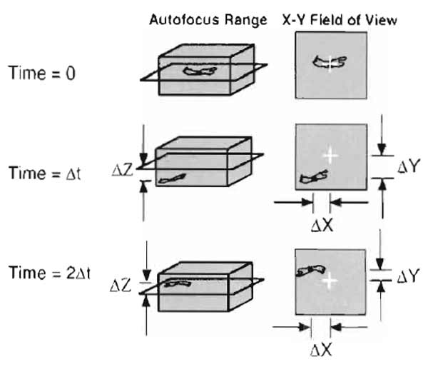 |
| FIGURE 5 Schematic of autofocus and cell-tracking scheme for high magnification tracking in 3D. Initially, cells are focused and positioned in the center of the field of view. At the next time interval, the computer-controlled stage and focus move to the previously recorded position and execute an autofocus routine to locate the cell and determine the distance moved in the Z direction. A snapshot is taken, the centroid of the cell is located, and the X and Y distances moved by the cell are recorded. The process is repeated for the next and subsequent intervals, always returning the stage to the centroid recorded at the previous interval for each cell. |
A. Correcting cell tracks
- Subtract initial position for each object from subsequent positions for that object. Each object should now begin at 0,0,0.
- Subtract the XYZ position of the bead from XYZ colocalized cells for each time interval.
- Write a new file of corrected object positions.
B. Calculating MSD
| MSD = Δx2 + Δy2 + Δz2 | (3) |
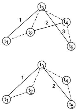 |
| FIGURE 6 Overlapping vs nonoverlapping intervals for calculating mean-squared displacement (MSD). In this example, an object is imaged five times (t1-t5) over four time intervals. Suppose we are determining the MSD over two time intervals. With the overlapping interval procedure (top), the distance traveled by the object during two time intervals can be measured three times (solid lines), whereas with the nonoverlapping technique, the same measurement can only be made twice. |
In an MSD calculation, we generate X-Y data that address the question: How far did an object, on average, migrate over a time interval of a given duration? In analyzing cell migration, we assume that cells have no inertia. That is, the fact that a cell is moving at a particular speed in a particular direction at time 1 has no assumed influence on the speed or direction at time 2, or any future time. Therefore, to determine the average distance traveled by a cell over one time interval, we average all displacements that occurred over 1 time interval. Thus, if the time lapse were four intervals long (five time points), we would calculate:
From t = l to t = 2: MSD1
From t = 2 to t = 3: MSD2
From t = 3 to t = 4: MSD3
From t = 4 to t = 5: MSD4
MSD for 1 time interval = average (MSD1-4)
We then average these over all of the cells in a given condition to arrive at the MSD value for that number of time intervals.
The use of overlapping vs nonoverlapping intervals arises when calculating the MSD over durations greater than I time interval (Fig. 6). For instance, in the example just given, if we want to calculate the MSD that occurs over 2 time intervals, we have two choices:
Option 1: Overlapping intervals
From t = l to t = 3: MSD1
From t = 2 to t = 4: MSD2
From t = 3 to t = 5: MSD3
Option 2: Nonoverlapping intervals
From t = l to t = 3: MSD1
From t = 3 to t = 5: MSD2
The MSD should be calculated for all possible interval durations. Again, using our 5 time point, 4 interval example and assuming overlapping intervals we would have
Over 1 time interval: MSD1 = average of 4 MSD measurements (1-2, 2-3, 3-4, 4-5)
Over 2 time intervals: MSD2 = average of 3 MSD measurements (1-3, 2-4, 3-5)
Over 3 time intervals: MSD3 = average of 2 MSD measurements (1-4, 2-5)
Over 4 time intervals: MSD4 = 1 MSD measurement (1-5)
X-Y data are then generated as follows
| X = duration | Y = average MSD over that number of intervals |
| 1 Δt | MSD1 |
| 2 Δt | MSD2 |
| 3 Δt | MSD3 |
| 4 Δt | MSD4 |
A full time-lapse experiment would include many more intervals and therefore a much greater amount of data.
C. Fitting data to the random walk model. The easiest way to fit data is to use a program (or write one yourself) capable of nonlinear regression. Fit X-Y data to Eq. (2) to identify µ and P (or S and P). If a nonlinear regression package is not available, the parameters can be estimated by recognizing that the MSD vs duration plot can be separated into two distinct regions: at short durations, the curve goes as time2, with slope ~ndS2, and at long durations the curve goes as time, with slope ~2ndµ. An investigator can split MSD curves into these two regions and then use standard linear regression to identify cell traction parameters.
Finally, Shreiber et al. (2003) have detailed a technique to temporally resolve mean-squared displacement data.
- Do not trust that all objects are tracked appropriately. Review time-lapse movies of each experiment and note which objects are lost or switched to a different object and disregard these cells in data analysis.
- Equation (2) assumes that cells move randomly. If it appears that cells are not moving randomly, examine the cell tracks of individual cells (look at all, not just a few) to visually inspect for any directional bias. Also, mean-squared displacement data can be generated for one direction at a time and the MSD in each direction independently fit to Eq. (2). If the migration is indeed random, then cell migration parameters should be (within error) the same for analysis of the X direction, the Y direction, and the Z direction.
- Note that in calculating values for MSD, more measurements go into calculating the average MSD over one interval than over two intervals, more over two than over three intervals. Thus, there is generally more error in the calculation of MSD over long durations than short durations. This can be accounted for in the analysis by repeating data for a given duration to represent the number of samples that were included in the average calculation.
- The increase in error in the MSD calculation over long durations can also produce aberrant behavior in the MSD plot. Specifically, the MSD plot may deviate from linear behavior as the error in the MSD calculation increases. These points can be ignored in processing data.
The combined migration/traction assay allows assessment of the contractile ability of cells and their motility (Knapp et al., 2000; Shreiber et al., 2001, 2003). It is more technically challenging than either assay is individually and requires machining of special chambers. A schematic of the chamber is shown in Fig. 7, but the dimensions are somewhat arbitrary and can be tuned to the specific need of the investigator. Our assay chamber consists of a stainless-steel annulus (2.5 cm o.d., 1.5 cm i.d., 0.6cm thick) with 3-mm holes located 1 mm from the bottom surface, bored through the side of the annulus. For stressed gel assays, two stainless-steel posts (3 mm diameter, 1.2 and 0.8cm in length) with flared ends fit securely into opposing holes. On the inside ends of the two posts is glued a 3- mm-diameter, 1-mm-thick disk of porous polyethylene. A polycarbonate tube with an inner diameter matching the diameter of the posts/disks is supported by the two posts and serves as a mold for the assay. When the tube is filled with a collagen or fibrin solution, the solution penetrates the pores to form a fixed boundary condition upon gel formation. For unstressed, free-floating gels, the stainless-steel posts are replaced with polycarbonate posts that are each 1 mm longer to account for the lack of a porous polyethylene disk. In these cases, the gel forms without a rigid attachment, and the gel is free to compact uniformly in all directions.
 |
| FIGURE 7 Individual components of a single traction/migration chamber. The stainless-steel posts and porous polyethylene discs are used in the stressed, constrained assay. The polycarbonate posts are used in the unstressed, free floating assay and are slightly longer to accommodate the length lost by not including the porous polyethylene. |
- Prepare collagen or fibrin solution as described earlier. Be sure to degas the collagen/fibrin.
- Add cells to desired concentration (7500-30,000 cells/ml).
- Add beads (7500-10,000beads/ml).
- Prepare culture medium with defined soluble factors of interest (e.g., 50ng/ml PDGF).
- Under sterile conditions, hold the assay chamber in one hand with the sheath supported by one post. Fill the sheath with the gel solution from steps 1-3.
- Gently push the opposing post into the mold.
- With vacuum grease, secure a coverslip to the top and bottom of the chamber and place in an incubator.
- Gently flip the chamber every 5 min until the solution is gelled to prevent cells and beads from settling to the bottom.
- Remove chamber from incubator, place right side up, and carefully remove the top coverslip.
- Fill the chamber with medium from step 4.
- With sterile tweezers, gently slide the sheath over the long post to expose gel to culture medium.
- Replace the coverslip, again securing with vacuum grease.
- Transfer chambers to microscope stage and prepare tracking algorithm (section VIII,A).
A schematic of the final steps is provided in Fig. 8.
 |
| FIGURE 8 Schematic of cell traction/cell migration assay preparation. Fill the polycarbonate sheath with the biopolymer solution (+cells and beads) and support with stainless-steel posts, use vacuum grease to cover top and bottom surfaces with glass coverslips, and transfer to the incubator to facilitate gelation. After gelation, remove the top coverslip and fill the chamber with culture medium with defined concentrations of soluble factors of interest. Slide the sheath over the long post to expose the gel to the culture medium. Replace the top coverslip and transfer to the microscope stage for traction and migration tracking. |
A. Microscopy
The migration/traction assay requires at least an XY motorized stage. Automated focus is preferred and rotating objectives are ideal. The routines for tracking cell migration are identical to those described previously. To record cell traction, follow initial selection of cell/bead positions, move the stage to the center of each chamber, and instruct the computer to build a mosaic image of the gel at the midplane. This is done most easily with a low power objective; if available, use the motorized objective feature to switch objectives to 2 or 4X. This process should be repeated automatically at the end of each time interval. A typical time lapse is run for 12-48h. Typical "before" and "after" images of the stressed and unstressed assays are shown in Fig. 9.
 |
| FIGURE 9 Examples of unstressed, free-floating assay (A,C) and stressed, constrained assay (B,D). Migration-traction assays are prepared as described and are nearly identical after initial preparation. (A) Free-floating cylindrical gel at time = 0. The gel was formed by supporting a sheath with smooth-ended polycarbonate posts. (B) Contstrained cylindrical gel at time = 0. The gel was prepared by filling an identical sheath that is supported by stainless-steel posts with porous polyethylene discs glued to the ends (outside field of view). The biopolymer solution penetrates the pores to form a fixed boundary condition upon gelation. Following incubation, cells that are entrapped in the gel exert traction and compact the gel. (C) Without physical constraints to compaction, the free-floating, cylindrical gel compacts (roughly) uniformly. (D) In contrast, the physical connection to the posts via the porous polyethylene prevents the constrained gel from compacting in the axial direction. The result is pure radial compaction and subsequent fiber and cell alignment. The characteristic "hourglass" shape results. In both cases, the degree of cell traction is related to the amount of gel compaction, measured as the decrease in radius at the midplane of the sample. |
Cell migration and traction analyses are performed as before. For traction, measure the diameter at the midplane of the gel at each time point. The fixed, stressed gel should form an hourglass during cellmediated gel compaction, so the diameter measurement should essentially be the middle of the hourglass. The free floating, unstressed gels should compact uniformly, so the diameter measurement can be taken from any cross-section. The result is X-Y data of percentage compaction vs time, which can be examined for temporal trends or quantified on the basis of final midplane compaction and compared to results of the migration analysis.
C. Pitfalls
- Be careful not to introduce bubbles into the assay that can affect gel compaction and obscure imaging.
- Similarly, do not smear vacuum grease over the coverslip in an area that will obscure imaging.
- Use hydrophilic porous polyethylene (Small Parts, Miami Lakes, FL) to ensure good penetration of the gel-forming solution for the fixed case.
- In the free-floating case, cell traction and/or convective motion of the culture medium may lead to rigid body motion of the cylindrical gel. Because cell migration may be tracked at high magnification, a small translocation of the gel can result in "losing" all of the cells during the traction algorithm, as it is only prepared to follow movements of 0.5 xFOV per interval. Use a low percentage, sterile, agarose solution (1%) to increase the viscosity of the culture medium and to reduce the ability for gel movement.
- Similarly, under some conditions (high cell concentration, certain concentrations of soluble factors, etc.), gels may compact too quickly to monitor cell position. Some trial and error is likely necessary to converge on appropriate conditions.
- Bubbles in the medium can also diminish imaging capabilities. Degas the culture medium and be careful when filling and sealing the chambers to avoid introducing air.
- Strong compaction in the stressed case leads to fiber alignment in the axial direction, which can lead to anisotropic migration. It may be necessary to quantify migration in the individual directions (X,Y, and Z) for these cases.
- Generally, because of the high variability in cell lines from culture to culture and passage to passage, it is recommended to run all experimental conditions in one set of experiments rather than running all controls one day, all at one condition the next, and so on.
Barocas, V. H., Moon, A. G., and Tranquillo, R. T. (1995). The fibroblast- populated collagen microsphere assay of cell traction force 2. Measurement of the cell traction parameter. J. Biomech. Engin. 117(2), 161-170.
Barocas, V. H., and Tranquillo, R. T. (1997a). A finite element solution for the anisotropic biphasic theory of tissue-equivalent mechanics: The effect of contact guidance on isometric cell traction measurement. J. Biomech. Engin. 119(3), 261-268.
Barocas, V. H., and Tranquillo, R. T. (1997b). An anisotropic biphasic theory of tissue-equivalent mechanics: the interplay among cell traction, fibrillar network deformation, fibril alignment, and cell contact guidance. J. Biomech. Engin. 119(2), 137-145.
Bell, E., Ivarsson, B., and Merrill, C. (1979). Production of a tissue-like structure by contraction of collagen lattices by human fibroblasts of different proliferative potential in vitro. Proc. Natl. Acad. Sci. USA 76(3), 1274-1278.
Clark, R. A. E (ed.) (1996). "'The Molecular and Cellular Biology of Wound Repair." Plenum Press, New York.
Dickinson, R. B., and Tranquillo, R. T. (1993). Optimal estimation of cell movement indices from the statistical analysis of cell tracking data. AIChE J. 39(12), 1995-2010.
Eastwood, M., et al. (1996). Quantitative analysis of collagen gel contractile forces generated by dermal fibroblasts and the relationship to cell morphology. J. Cell. Physiol. 166, 33-42.
Ehrlich, H. P., and Rajaratnam, J. B. (1990). Cell locomotion forces versus cell contraction forces for collagen lattice contraction: An in vitro model of wound contraction. Tissue Cell 22(4), 407-417.
Knapp, D. M., et al. (1997). Rheology of reconstituted type I collagen gel in confined compression. J. Rheol. 41(5), 971-993.
Knapp, D. M., Helou, E. E, and Tranquilllo, R. T. (1999). A fibrin or collagen assay for tissue cell chemotaxis: Assessment of fibroblast chemotaxis to GRGDSP. Exp. Cell Res. 247, 543-553.
Knapp, D. M., et al. (2000). Estimation of cell traction and migration in an isometric cell traction assay. AIChE J. 45(12), 2628-2640.
Kolodney, M. S., and Wysolmerski, R. B. (1992). Isometric contraction by fibroblasts and endothelial cells in tissue culture: A quantitative study. J. Cell Biol. 117(1), 73-82.
Neidert, M. R., et al. (2002). Enhanced fibrin remodeling in vitro with TGF-betal, insulin and plasmin for improved tissue-equivalents. Biomaterials 23(17), 3717-3731.
Nusgens, B., et al. (1984). Collagen biosynthesis by cells in a tissue equivalent matrix in vitro. Coil Relat Res. 4(5), 351-363.
Shreiber, D. I., Barocas, V. H., and Tranquillo, R. T. (2003). Temporal variations in cell migration and traction during fibroblast-mediated gel compaction. Biophys J. 84(6), 4102-4114.
Shreiber, D. I., Enever, P. A., and Tranquillo, R. T. (2001). Effects of pdgf-bb on rat dermal fibroblast behavior in mechanically stressed and unstressed collagen and fibrin gels. Exp. Cell Res. 266(1), 155- 166.
Tuan, T. L., et al. (1996). In vitro fibroplasia: Matrix contraction, cell growth, and collagen production of fibroblasts cultured in fibrin gels. Exp Cell Res. 223(1), 127-134.
Support our developers