Assessment of Critical Nutrient Values

Critical values are indispensable for evaluating the nutritional status of a crop. Important threshold markers are: (a) the symptomatological value, which reflects the sulfur concentration below which deficiency symptoms become visible (see Section); (b) the critical nutrient value, which stands for the sulfur concentration above which the plant is sufficiently supplied with sulfur for achieving the maximum potential yield or yield reduced by 5, 10, or 20% (294); and (c) the toxicological value, which indicates the sulfur concentration above which toxicity symptoms can be observed. However, there is no one exclusive critical nutrient value for any crop, as it depends on the growth conditions, the developmental stage of the plant at sampling, the collected plant part, the determined sulfur species, the targeted yield, and the mathematical approach for calculating it. Smith and Loneragan (295) provided a comprehensive, general overview of the significance of relevant factors influencing the derivation of critical values. Numerous, differing critical sulfur values and ranges exist for each crop and have been compiled, for instance by Reuter and Robinson (294), for all essential plant nutrients and cultivated plants including forest plantations. In this section, an attempt was made to compile and categorize, from the literature, available individual data based on studies with varying experimental conditions of the variables, total sulfur and sulfate concentrations, and N/S ratios in relation to different groups of crops for facilitating an easy and appropriate evaluation of sulfur supply. Plant groups were assembled by morphogenetic and physiological features. Because of the wide heterogeneity of results for similar classes of sulfur supply and for a better comparability of results, concentrations were agglomerated into three major categories: deficient, adequate, and high, irrespective of the sampled plant part during vegetative growth (Table 7.6). A prior-made subdivision, which took these relevant criteria into consideration (see Section) next to additional characteristics of the sulfur supply (symptomatological and critical values of total S, sulfate, and N/S ratio), did not prove to be feasible as the variation of results was so high that no clear ranges, let alone threshold values, could be assigned for individual classes and crops, or crop groups.

Smith and Loneragan (295) stressed that in addition to various biotic and abiotic factors, experimental conditions, plant age, and plant part, all influence the nutrient status; the procedure to derive a critical value itself has a significant impact, so that it is possible to define only ranges for different nutritional levels. This finding also implies that it is more or less impossible to compare results from different experiments. The integration of individual studies, which imply extreme values, are not suitable for a generalization of an affiliation to a certain class of sulfur supply and, more importantly, such interpretation may even yield an erroneous evaluation of the sulfur supply. In comparison, the compilation of the data in Table 7.6 indicates that the sampled plant part during the main vegetative development seems to be of minor relevance for generally addressing the sulfur nutritional status. However, for following up, for instance, nutritional or pathogen-related changes in sulfur metabolism, it might even be necessary to do so in defined parts of a plant organ or on a leaf cell level.

TABLE 7.6

Mean Critical Values and Ranges of Sulfur Nutrition for Different Groups of Agricultural Crops

Click to view the table (Approx. 431KB) (opens in new window)

Download the clear image of the table to view offline (Approx. 1.02MB .zip file)

The results in Table 7.6 reveal that Poaceae and fodder crops have been studied intensely in relation to sulfur nutritional supply. For all crops, the total sulfur concentration was used most often to characterize the sulfur nutritional status. The range of variation was distinctly lower for total sulfur than for sulfate concentrations, independent of the crop type. It is also remarkable that the ranges in the three classes overlap regularly for all groups of crops and sulfur fractions. With the exception of the fodder crops, however, the 25 and 75% quartiles separate samples from the three nutritional levels efficiently if total sulfur concentrations were determined. For sulfate, such partition was feasible too, except in Poaceae. Generally, an insufficient sulfur supply is indicated by total sulfur concentrations of <1.7 mg g^-1. In the case of Poaceae and nonbrassica vegetables, this value may be lower at 0.94 mg S g^-1 or higher at 2.9 mg S g^-1 (Table 7.6). Sulfate concentrations of <150mg SO₄-S kg^-1 indicate an insufficient sulfur supply. An adequate sulfur supply is reflected by total sulfur concentrations of 1.7 to 4 mg S g^-1; brassica crops show a higher optimum range with values of 4.8 (oil crops) to 7.5 (vegetables) mg S g^-1 (Table 7.6). Values of 16 to 20 for N/S ratio, and 150 to 1600 for sulfate-S concentrations reflect a sufficient sulfur supply. In comparison, values of 2800mg SO₄-S kg^-1 denote an excessive sulfur supply (Table 7.6). Sulfate is usually not determined in brassica oil crops and vegetables as the degradation of glucosinolates might falsify the result. For fodder crops, total sulfur concentrations of even 3.2 mg S g^-1 may be disproportionate, whereas the corresponding value for nonbrassica vegetables would equal 10 mg S g^-1.

The major criticism of critical values for the interpretation of tissue analysis is the small experimental basis, which often consists of not more than a single experiment (297). Besides the lack of data, the method of interpretation may also yield erroneous results. Methods based on regression analysis, like the 'broken stick method' by Hudson (298) and Spencer and Freney (241), or the 'vector analysis' by Timmer and Armstrong (299) investigate mathematical, but not necessarily causal, interactions between the nutrient content and yield, because the dictate of minimizing the sum of squared distances aims only to find a function that fits best across the data set. Like the method of Cate and Nelson (300,301), these methods have been designed primarily for the investigation of small data sets and plants grown under ceteris paribus conditions, where only the response to variations in the nutrient supply varied. Another quite significant disadvantage of critical values and critical ranges(Tissue concentration for 95% of maximum yield.) (143,296,302), or 'no-effect values (NEV)(Tissue concentration for maximum yield or the concentration above which no yield response occurs.) (284) is that they ignore the nonlinearity of the Mitscherlich function describing the relationship between growth factors and yield (303). The ideal basis for critical values for the interpretation of tissue analysis are large sets of yield data and nutrient concentrations in defined plant organs that cover a wide range of growth factor combinations. The data may include samples from field surveys or field or pot experiments if the reference yield of 100% was obtained in all cases under optimum growth conditions. In Figure 7.15 and Figure 7.16, corresponding examples are given for the total sulfur concentration in shoots of cereals at stem extension and the N/S ratio in younger, fully developed leaves of oilseed rape at stem extension.

The data in Figure 7.15 reveal a characteristic bow-shaped bulk, which covers sulfur concentrations from 0.5 to 5.5 mg S g^-1. Sulfur deficiency can be expected at sulfur concentrations below 0.94 mg g^-1 (Table 7.6). A symptomatological threshold for the expression of macroscopic symptoms of 1.2 mg S g^-1 was determined for cereals by Schnug and Haneklaus (114). Total sulfur concentrations of 1.7 mg g^-1 are considered as being adequate to satisfy the sulfur demand of cereal crops, whereas the data in Figure 7.15 show a further yield increase with higher sulfur concentrations. The reason is simply that the 100% yield margin corresponds to a grain yield of 10 t ha^-1 (180), so that accordingly a total sulfur concentration of 1.7 mg S g^-1 would be sufficient for 8.2 t ha^-1. A productivity level of 10 t ha^-1 is extraordinarily high and restricted to areas of high fertility or inputs, whereas a level of 8 t ha^-1 represents a high-yielding crop in many areas in the world. Thus, a total sulfur concentration of 4.7 mg g^-1, which is rated as reflecting a high sulfur supply, is marginal on high productivity sites.

Basic shortcomings of using, for instance, the N/S ratio for the evaluation of the sulfur nutritional status were discussed and are reflected in the data in Figure 7.16. Hence, there are no relationships between N/S ratio and yield in a way as was shown for total sulfur and cereals (Figure 7.15). Crop productivity seems to be fairly independent of variations in the N/S ratio within a range of 5:1 to 12:1 (Figure 7.16).

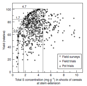FIGURE 7.15 Scattergram of total sulfur in shoots and yield data for cereals in relation to experimental conditions (From Schnug, E. and Haneklaus, S., in Sulphur in Agroecosystems. Vol. 2, Part of the series 'Nutrients in Ecosystems', Kluwer Academic Publishers, Dordrecht, 1998, pp. 1-38.) and merged values thresholds for sulfur supply.

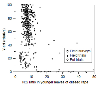FIGURE 7.16 Relationship between N:S ratio in young leaves of oilseed rape at stem extension and relative seed yield. (From Schnug, E., Quantitative und Qualitative Aspekte der Diagnose und Therapie der Schwefelversorgung von Raps (Brassica napus L.) unter besonderer Ber�cksichtigung glucosinolatarmer Sorten. Habilitationsschrift, D.Sc. thesis, Kiel University, 1988.)

Comprehensive data sets like those presented in Figure 7.15 allow for the accurate calculations of so-called upper boundary line functions, which describe the highest yields observed over the range of nutrient values measured. Data points below this line relate to samples where some other factor limited the crop response to the nutrient. An overview of the scientific background and development of upper boundary lines is given by Schnug et al. (304).

The Boundary Line Development System (BOLIDES) was elaborated to determine the upper boundary line functions and to evaluate optimum nutrient values and ranges. The BOLIDES is based on a five-step algorithm (Figure 7.17) (304). For the identification of outliers, cell sizes are defined for nutrient and yield values together with an optional number of data points per cell (Figure 7.17a). The cell size can be chosen variably with proposed values for X (nutrient content) corresponding to the standard deviations and for Y (yield) with the coefficient of variation. If another variable, often a stable soil feature such as organic matter or clay content, has a significant effect on the response to the nutrient, its presence is indicated by two or more distinct concentrations of points, each with its own boundary line response to the nutrient (Figure 7.17b). The data can be classified on the basis of this third variable, and the boundary line can be determined separately for each class. Next, a boundary step function is calculated for each class, starting from the minimum nutrient content up to the point of maximum yield, as well as from the maximum nutrient content up to the maximum yield (Figure 7.17c). Then the boundary line, usually a first-order polynomial function, is fitted according to the least-squares method (Figure 7.17d). The first derivative of the fitted polynomial gives predicted yield response to fertilization in relation to the nutrient content (Figure 7.17). The last step is the classification of the nutrient supply to determine optimum nutrient levels or optimum nutrient ranges. The optimum nutrient value corresponds with the zero of the first derivative of the upper boundary line and the sign of the second derivative at this point. For the determination of the optimum ranges, that is, the range of nutrient concentration that gives 95% of the maximum yield, standard, numerical root-finding procedures are used for real polynomials of degree 4 with constant coefficients (Figure 7.17).

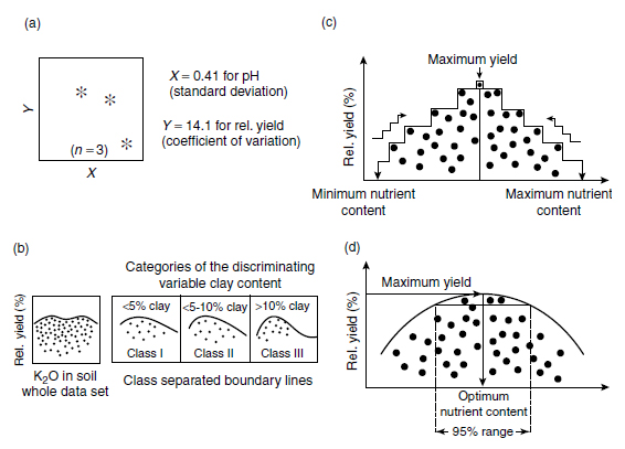FIGURE 7.17 Structure of Boundary Line Development System (BOLIDES) for the determination of upper boundary line functions and optimum nutrient values and ranges in plants and soils: (a) identification of outliers; (b) discrimination against a third variable; (c) calculation of step functions; and (d) determination of the upper boundary line and calculation of optimum nutrient value and ranges. (From Haneklaus, S. and Schnug, E., Aspects Appl. Biol., 52, 87-94, 1998.)

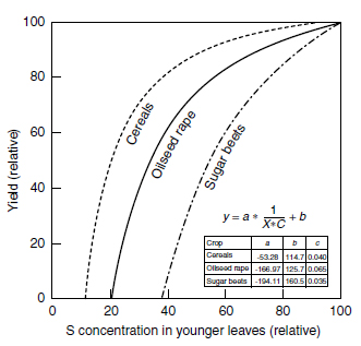FIGURE 7.18 Comparison of boundary line functions for yield and total sulfur concentration in tissue of cereals, oilseed rape, and sugar beet. (From Schnug, E. and Haneklaus, S., in Sulphur in Agroecosystems, Vol. 2, Part of the series 'Nutrients in Ecosystems', Kluwer Academic Publishers, Dordrecht, 1998, pp. 1-38.)

Thus boundary lines describe the 'pure effect of a nutrient' on crop yield under ceteris paribus conditions (246,247,305,306). The comparison of the boundary lines for total sulfur and yield (both relative) for oilseed rape, cereals, and sugar beet (Figure 7.18) reveals the physiological differences between these crops. The boundary lines for cereals and oilseed rape are for seed yields, and that for sugar beet for root yields. The optimum sulfur ranges proved to be the same for sugar beet root yield and sugar yield.

For all crops, the boundary lines show a steep increase at the beginning, which reflects the response of the photosynthetic system to sulfur deficiency. In cereals, the boundary line continues over a long range and asymptotically toward the value above which no further yield increase (NEV) is to be expected from increasing sulfur concentrations. This part of the boundary line most likely reflects the proportion of sulfur that is bound to the proteins of the cereal grain. In sugar beet, the boundary line reaches the NEV much faster after a steep increase, which is in line with the fact that sugar beet roots take up only small amounts of sulfur (205). Oilseed rape, with its internal storage system for S, which is based on the enzymatic recycling of glucosinolates (90,289), shows a steadier ascent of its boundary line. Therefore, within oilseed rape varieties, those with genetically low glucosinolate contents ('double low' or '00' varieties) show a steeper increase of their boundary lines than those with genetically high glucosinolate concentrations (103,116).

The nonlinearity of the boundary lines reveals once more the limited value of critical values. Above total sulfur concentrations of 6.5, 4.0, and 3.5 mg g^-1 in foliar tissue of oilseed rape, cereals, and sugar beet, respectively, no further yield increases are to be expected by increasing tissue sulfur concentrations (NEVs). This result corresponds to the usually assigned 'critical values,' which are valid for 95% of the maximum yield, of 5.5, 3.2, and 3.0 mg S g^-1 for rape, corn, and sugar beets, respectively. However, in this range of the response curve, there is still no linearity between tissue sulfur levels and yield.

The relationship between sulfur concentration in plant tissue and yield, which reflects the physiological patterns in the internal nutrient utilization, is specific for each plant species, and can be best established by boundary lines (Figure 7.17). In comparison, the relationship between fertilizer dose and sulfur concentration in plant tissues is much less dependent on physiological factors but is strongly influenced by factors affecting the physical mobility and losses of sulfur from soils. Therefore, this transfer function bears the largest part of insecurity for the effectiveness of sulfur fertilization. Thus, for the derivation of fertilizer recommendations, the common relationship between fertilizer dose and yield is best split into two partial relationships: (a) fertilizer dose versus nutrient uptake and (b) nutrient uptake versus yield (307). If tissue analysis is to be used for fertilizer recommendations, concentrations need to be calibrated against sulfur doses. This strategy was proved for nitrogen (308), and the setting up of sulfur response curves is recommended for sulfur too.

Professional Interpretation Program for Plant Analysis (PIPPA) software not only evaluates the status of individual plant nutrients but also appraises results from multiple elemental analyses (309). In PIPPA, boundary line and transfer functions are integrated for each element so that the yieldlimiting effect is calculated for each specified nutrient, and finally fertilizer recommendations are given (309).