Chi-square test

The chi square (χ²) test for segregation ratios and detection of linkage
In the beginning of this section, we described two examples of linkage, one each in sweet pea and maize, where results of a dihybrid test cross (AaBb x aabb) deviated from 1AB : 1Ab : 1aB : 1ab ratio expected due to independent assortment. In experiments like these, when there are deviations from expected 1:1:1:1 ratio or 9 : 3 : 3 : 1 ratio, it may not be easy to decide on the presence or absence of linkage by simply looking at the data. Instead an analytical approach may be needed. The chi-square (χ²) test is one such approach, which is used firstly, for testing the goodness of fit to an expected ratio and secondly, for the detection of linkage in more certain terms. This test tells us how often deviations like those being examined will occur purely on the basis of chance.

χ² Test for goodness of fit. Following steps are involved in a chi-square test. They will be illustrated for χ² test for goodness of fit but are also used for the other two χ² tests (χ² tests for independence and homogeneity) described later. (a) Formulate a null hypothesis. Good fit to expected 1:1:1:1 ratio or 9 : 3 : 3 : 1 ratio are examples of null hypothesis used to test the fitness of given data to these ratios.

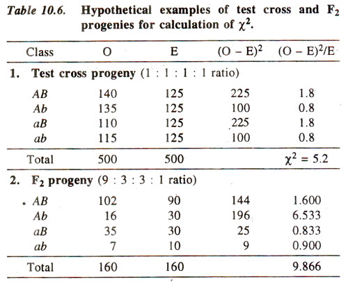
(ii) Calculate χ². This value is calculated from observed (O) results, using actual numbers (not from percentages or fractions) and expected (E) results calculated from total population using 1:1:1:1 ratio or 9 : 3 : 3 : 1 ratio (whichever is the case). Following formula is used :



(where σ refers to sum of values of χ², over all classes) The use of this formula for test cross progeny (1:1:1:1 ratio) and F₂ progeny (9:3:3:1 ratio) is illustrated in Table 10.6.

(iii) Work out degrees of freedom. The degrees of freedom (df) can be worked out as follows :

df = (number of classes - 1)

In the above examples df = (4 - 1) = 3 (iv) From χ² table, probability of getting the computed value of χ²is read (see Table 10.8). In the examples shown in Table 10.6, the probabilities of getting χ² value of 5.2 and 9.866 for 3 degrees of freedom as drawn from Table 10.8 are between 0.1 and 0.2 (or between 10% to 20%) and between 0.05 to 0.01 (below 5% and above 1%) respectively.

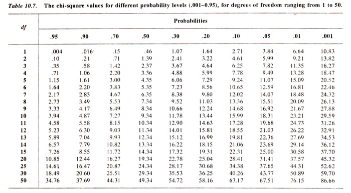
(v) Reject or accept the null hypothesis. We generally use an arbitrary value of p = 0.05 = 5%, so that if the computed value of χ². is below 5% level of probability, we reject the null hypothesis, otherwise accept it. In the examples as above, for test cross progeny, χ² = 5-2 has a p > 10%. Therefore, null hypothesis is accepted, suggesting that the ratio 1:1:1:1 holds good. On the other hand, for F₂ progeny, χ² = 9.866 has a p < 5% suggesting that the ratio 9:3:3:1 does not hold good.

χ² test for independence (linkage). The chi-square (χ²) value for three degrees of freedom obtained for goodness of fit to 1 : 1 : 1 : 1 or 9:3:3:1 ratio can be further partitioned into χ² values for individual degrees of freedom. In a dihybrid AaBb, while analysing testcross data or F₂ data, the three values of χ² obtained from such partitioning, can be individually used, one each to test the following : (i) departure from 3A : 1a ratio; (ii) departure from 3B : 1b ratio and (iii) departure from independent assortment of A and B, due to linkage. It is obvious thus that a deviation from an expected 9:3:3:1 or 1:1:1:1 ratio may not be necessary due to linkage, but may instead be due to distortion in the segregation at A vs. a locus or B vs. b locus (due to lack of full viability of the recessive phenotype). Rarely, it is also possible that the χ² value for three degrees of freedom is not significant, but one of the three χ²values (each for single degree of freedom) is significant, showing either distortion at one locus or lack of independence (presence of linkage). The above can be explained using data from two examples used in Table 10.6.

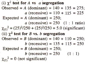
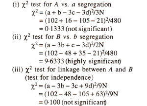
Partitioning of χ² value for a dihybrid test cross progeny. The χ² value of 5.2 for 3 degree of freedom obtained in Table 10.6 for 1 : 1 : 1 : 1 ratio can be partitioned as follows :


(iii) χ² test for independence
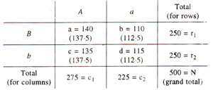
For this test, expected ratios are not available, but expected values for each class can be calculated, assuming that segregation at one locus (A vs. a) is not dependent (contingent) upon the segregation at the second locus (B vs. b). The test is called 'test for independence or contingency test'. For conducting this test, the data from Table 10.6, is rearranged in a contingency table as follows :



where,
a = AB r₁ = first row total
b = aB r₂ - second row total
c = Ab c₁ = first column total
d = ab c₂ = second column total

degrees of freedom for χ² = (r - 1) (c - 1) = 1

(r = number of rows; c = number of columns)

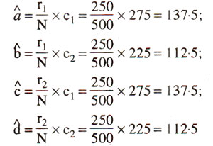
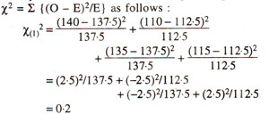
In the above contingency table, the expected values (a^,b^,c^,d^) of a, b, c, and d are given in parentheses and can be calculated as follows :



Using observed and expected values, the chi-square can be calculated using the equation, χ² = Z {(O - E)²/E} as follows :



The chi-square for independence can also be calculated using the following equation, so that expected values need not be calculated.


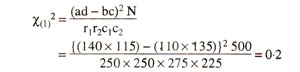
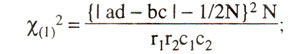
However it is recommended that, when any one of the four observed values (a, b, c, d) is below 5, a Yate's correction for continuity should be applied, and the equation is modified as follows :



In | ad - be |, vertical lines mean that this value will always be taken as positive, even when it is negative

The above partitioning of χ² demonstrates clearly that although there is a good fit to the ratio 1:1:1:1, but there is some distortion in segregation of A vs. a, and that there is no evidence of linkage.

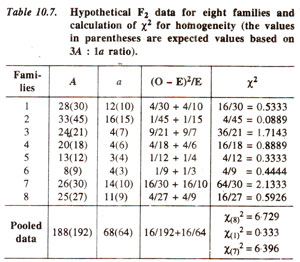
Partitioning of χ² value for a dihybrid F₂ population. The chi-square value for goodness of fit to 9 : 3 : 3 : 1 ratio expected in F₂ population derived due to selfing of a F₁ dihybrid (AaBb) can also be partitioned. As an illustration, the chi-square value of 9.866 for three degrees of freedom calculated for 9:3:3:1 ratio in Table 10.6 is significant at 5% level. This can be partitioned as follows :



For the above test for independence (F₂ data), one can also arrange the data in a contingency table and apply contingency test for one degree of freedom as done earlier for test cross data. In either case, you will notice that there is a distortion in the segregation for B vs. b, which leads to poor goodness of fit, but there is no evidence of linkage.



χ² test for homogeneity. This test is used, when the data from several individual similar experiments are desired to be pooled. In Table 10.7, data for 3 : 1 segregation from eight families are presented and χ² values calculated for each of them. The χ² value is also calculated for pooled data and subtracted from the sum of the individual χ² values for eight families. The balance χ² for seven degrees of freedom is used to test for homogeneity. From Table 10.8, one can see that the probability of getting a χ² of 6.396 is > 0.30 (>30%). Therefore it is concluded that the data is not heterogeneous and can be pooled.