Quantitative Variation
Quantitative Variation
Quantitative traits are those that show
continuous variation with no obvious
pattern of Mendelian segregation in
their inheritance. The values of the trait
in offspring often are intermediate
between the values in the parents.
Such traits are influenced by variation
at many genes, each of which follows
Mendelian inheritance and contributes
a small, incremental amount to the
total phenotype. Examples of traits that
show quantitative variation include tail
length in mice, length of a leg segment
in grasshoppers, number of gill rakers
in sunfishes, number of peas in pods,
and height of adult males of the
human species. When the values are
graphed with respect to frequency distribution,
they often approximate a
normal, or bell-shaped, probability
curve (Figure 6-31A). Most individuals
fall near the average; fewer fall somewhat
above or below the average, and
extremes form the “tails” of the frequency
curve with increasing rarity.
Usually, the larger the population sample,
the more closely the frequency
distribution resembles a normal curve.
Selection can act on quantitative traits to produce three different kinds of evolutionary response (see Figure 6-31B, C, and D). One outcome is to favor average values of the trait and to disfavor extreme ones; this outcome is called stabilizing selection (Figure 6-31B). Directional selection favors an extreme value of the phenotype and causes the population average to shift toward it over time (Figure 6-31C). When we think about natural selection producing evolutionary change, it is usually directional selection that we have in mind, although we must remember that this is not the only possibility. A third alternative is disruptive selection in which two different extreme phenotypes are simultaneously favored, but the average is disfavored (Figure 6-31D). The population will become bimodal, meaning that two very different phenotypes will predominate.
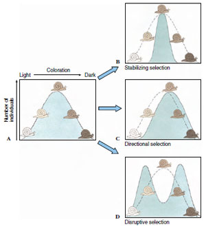 |
| Figure 6-31 Responses to selection on a continuous (polygenic) character, coloration in a snail. A, The frequency distribution of coloration before selection. B, Stabilizing selection culls extreme variants from the population, in this case eliminating individuals that are unusually light or dark, thereby stabilizing the mean. C, Directional selection shifts the population mean, in this case by favoring darkly colored variants. D, Disruptive selection favors both extremes but not the mean; the mean is unchanged but the population no longer has a bell-shaped distribution of phenotypes. |
Selection can act on quantitative traits to produce three different kinds of evolutionary response (see Figure 6-31B, C, and D). One outcome is to favor average values of the trait and to disfavor extreme ones; this outcome is called stabilizing selection (Figure 6-31B). Directional selection favors an extreme value of the phenotype and causes the population average to shift toward it over time (Figure 6-31C). When we think about natural selection producing evolutionary change, it is usually directional selection that we have in mind, although we must remember that this is not the only possibility. A third alternative is disruptive selection in which two different extreme phenotypes are simultaneously favored, but the average is disfavored (Figure 6-31D). The population will become bimodal, meaning that two very different phenotypes will predominate.
Support our developers