Choosing a suitable statistical test

Comparing location (e.g, means)
If you can assume that your data are normally distributed, the main test for comparing two means from independent samples is Student's t-test (see Boxes 41.1 and 41.2, and Table 41.2). This assumes that the variances of the data sets are homogeneous. Tests based on the t-distribution are also available for comparing paired data or for comparing a sample mean with a chosen value.

When comparing means of two or more samples, analysis of variance (ANOVA) is a very useful technique. This method also assumes data are normally distributed and that the variances of the samples are homogeneous. The samples must also be independent (e.g. not sub-samples). The nested types of ANOVA are useful for letting you know the relative importance of different sources of variability in your data. Two-way and multi-way ANOVAs are useful for studying interactions between treatments.

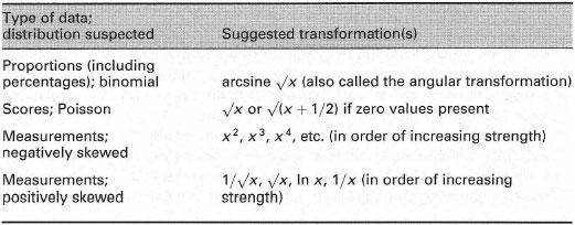Table 41. 1 Suggested transformations aIteri ng different types of frequency distribution to the normal type.

For data satisfying the ANOVA requirements, the least significant difference (LSD) is useful for making planned comparisons among several means. Any two means that differ by more than the LSD will be significantly different. The LSD is useful for showing on graphs.

The chief non-parametric tests for comparing locations are the Mann- Whitney U-test and the Kolmogorov-Smirnov test. The former assumes that the frequency distributions of the data sets are similar, whereas the latter makes no such assumption. In the Kolmogorov-Smirnov test, significant differences found with the test may be due to differences in location or shape of the distribution, or both.

Suitable non-parametric comparisons of location for paired quantitative data (sample size ≥ 6) include Wilcoxon's signed rank test, which assumes that the distributions have similar shape.

Non-parametric comparisons of location for three or more samples include the Kruskal-Wallis H-test. Here, the two data sets can be unequal in size, but again the underlying distributions are assumed to be similar.

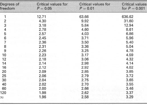Table 41.2 Critical values of Student's t statistic (for two-tailed tests). Reject the null hypothesis at probability P if your calculated t value exceeds the value shown forthe appropriate degrees of freedom = (n1 − 1) + (n2 − 1)

Comparing dispersions (e.g, variances)
If you wish to compare the variances of two sets of data that are normally distributed, use the F-test. For comparing more than two samples, it may be sufficient to use the F_max-test, on the highest and lowest variances. The Scheffe-Box (log-ANOVA) test is recommended for testing the significance of differences between several variances. Non-parametric tests exist but are not widely available: you may need to transform the data and use a test based on the normal distribution.

Determining whether frequency observations fit theoretical expectation
The χ²-test is useful for tests of 'goodness of fit', e.g. comparing expected and observed progeny frequencies in genetical experiments or comparing observed frequency distributions with some theoretical function. One limitation is that simple formulae for calculating χ² assume that no expected number is less than five. The G-test (2I test) is used in similar circumstances.
Comparing proportion data When comparing proportions between two small groups (e.g. whether 3/10 is significantly different from 5/10), you can use probability tables such as those of Finney et al. (1963) or calculate probabilities from formulae; however, this can be tedious for large sample sizes. Certain proportions can be transformed so that their distribution becomes normal.

Placing confidence limits on an estimate of a population parameter
On many occasions, sample statistics are used to provide an estimate of the population parameters. It is extremely useful to indicate the reliability of such estimates. This can be done by putting a confidence limit on the sample statistic. The most common application is to place confidence limits on the mean of a sample from a normally distributed population. This is done by working out the limits as Ÿ (Y bar) − (t_{P[n − 1]} × SE) and Ÿ (Y bar) + (t_{P[n − 1]} × SE) where t_{P[n − 1]} is the tabulated critical value of Student's t statistic for a two-tailed test with n − 1 degrees of freedom and SE is the standard error of the mean. A 95% confidence limit (i.e. P = 0.05) tells you that on average, 95 times out of 100, this limit will contain the population mean.


Regression and correlation
These methods are used when testing relationships between samples of two variables. If one variable is assumed to be dependent on the other then regression techniques are used to find the line of best fit for your data. This does not tell you how well the data fit the line: for this, a correlation coefficient must be calculated. If there is no a priori reason to assume dependency between variables, correlation methods alone are appropriate.

If graphs or theory indicate a linear relationship between a dependent and an independent variable, linear regression can be used to estimate the equation that links them. If the relationship is not linear, a transformation may give a linear relationship. For example, this is sometimes used in analysis of chemical kinetics. However, 'linearizations' can lead to errors when carrying out regression analysis: take care to ensure (i) that the data are evenly distributed throughout the range of the independent variable and (ii) that the variances of the dependent variable are homogeneous. If these criteria cannot be met, weighting methods may reduce errors. In this situation, it may be better to use non-linear regression using a suitable computer program.

Model I linear regression is suitable for experiments where a dependent variable Y varies with an error-free independent variable X and the mean (expected) value of Y is given by a + bX. This might occur where you have carefully controlled the independent variable and it can therefore be assumed to have zero error (e.g. a calibration curve). Errors can be calculated for estimates of a and b and predicted values of Y. The Y values should be normally distributed and the variance of Y constant at all values of X.

Model II linear regression is suitable for experiments where a dependent variable Y varies with an independent variable X which has an error associated with it and the mean (expected) value of Y is given by a + bX. This might occur where the experimenter is measuring two variables and believes there to be a causal relationship between them; both variables will be subject to errors in this case. The exact method to use depends on whether your aim is to estimate the functional relationship or to estimate one variable from the other.

A correlation coefficient measures the strength of relationships but does not describe the relationship. These coefficients are expressed as a number between −1 and 1. A positive coefficient indicates a positive relationship while a negative coefficient indicates a negative relationship (Fig. 41.6). The nearer the coefficient is to −1 or 1, the stronger the relationship between the variables, i.e. the less scatter there would be about a line of best fit (note that this does not imply that one variable is dependent on the other!). A coefficient of 0 implies that there is no relationship between the variables. The importance of graphing data is shown by the case illustrated in Fig.4l.6d.

Pearson's product-moment correlation coefficient (r) is the most commonly used correlation coefficient. If both variables are normally distributed, then r can be used in statistical tests to test whether the degree of correlation is significant. If one or both variables are not normally distributed you can use Kendall's coefficient of rank correlation (τ) or Spearman's coefficient of rank correlation (r_s). They require that data are ranked separately and calculation can be complex if there are tied ranks. Spearman's coefficient is said to be better if there is uncertainty about the reliability of closely ranked data values.

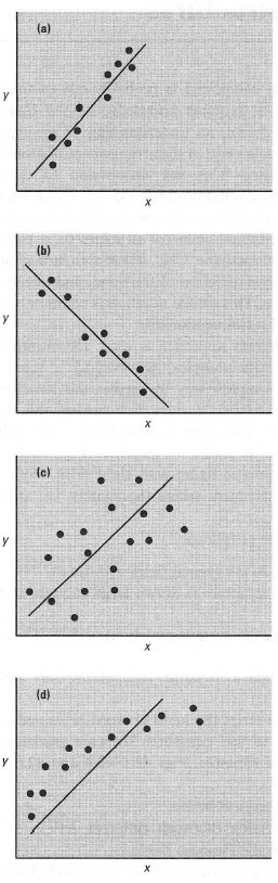Fig.41.6 Examples of correlation. The linear regression line is shown. In (a) and (b), the correlation between x and y is good: for (a) there is a positive correlation and the correlation coefficient would be close to 1; for (b) there is a negative correlation and the correlation coefficient would be close to −1. In (c) there is a weak positive correlation and r would be close to 0. In (d) the correlation coefficient may be quite large, but the choice of linear regression is clearly inappropriate.