Response surface methodology

Response surface methodology allows the relationship between the responses and variables to be quantified, using a mathematical model, and to be visualized. Thus the equation for a straight-line graph can be written as:

⇒ Equation [43.2]

y = mx + c

where m is a constant and c is the intercept. This describes the relationship between a single variable (x) and its response (y). Using the previous example, with three variables (x₁, x₂ and x₃) it is possible to extend this mathematical model.

First of all we can consider how each of the variables influences the response (y) in a linear manner. However, the relationship between y and x₁, x₂ and x₃ may not be linear, so it is necessary to consider the possibility of curvature. This is done in terms of a quadratic variable, i.e. a squared dependence (x_1², x_2² and x_3²). Finally, it is also important to consider the effects of possible interactions between the variables, x₁ → x₂ → x₃, i.e. x₁x₂, x₁x₃ and x₂x₃. The overall general equation can therefore be written as:

⇒ Equation [43.3]

Y = b0 + b1x1 + b2x2 + b3x3 + b4x12 + b5x22 + b6x32 + b7x1x2 + b8x1x3 + b9x2x3

where b₀ is the intercept parameter and b₁ − b₉ are the regression coefficients for linear, quadratic and interaction effects.

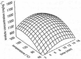Fig. 43.5 Example of a response surface.

This equation can be analysed using multiple linear regression and tested for statistical significance at, for example, the 95% confidence interval. In addition, the response can be explored by plotting a threedimensional graph. Unfortunately, in the above example, three variables are present. This immediately constrains what it is possible to plot on the graph (one of the axes must be the response). One way to select the two variables to plot is by considering their statistical significance and then selecting two variables which are significant at the 95% confidence interval. An alternative approach might be simply to plot the two variables you might wish to discuss in your experimental report. A typical response surface is shown in Fig. 43.5. It can be seen that the 'time' variable has a maximum at 8-12min while the 'temperature' variable has a maximum at l60-180°C. Further experiments might be carried out at these two maxima to determine the repeatability of the approach. However, it is necessary to plot all variables consecutively to identify all maxima.

In general, it is important to consider the following issues when carrying out an experimental design:

• Carry out repeat measurements for a particular combination of variables, to determine the repeatability of the approach.
• To remove systematic error (bias), you should randomize the order in which experiments are done.
• It is important to eliminate intervariable effects (confounding), i.e. the situation where one variable is inter-related to another.
• Often, the large number of experiments to be carried out makes it impossible to run all of them on the same day. If this happens run your experiments in discrete groups or 'blocks'.