Setting up a null hypothesis

Hypothesis-testing statistics are used to compare the properties of samples either with other samples or with some theory about them. For instance, you may be interested in whether two samples can be regarded as having different means, whether the concentration of a pesticide in a soil sample can be regarded as randomly distributed, or whether soil organic matter is linearly related to pesticide recovery.

*Note: You can't use statistics to prove any hypothesis, but they can be used to assess how likely it is to be wrong.

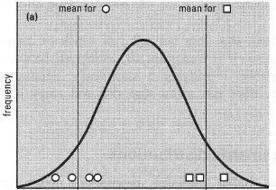
Statistical testing operates in what at first seems a rather perverse manner. Suppose you think a treatment has an effect. The theory you actually test is that it has no effect; the test tells you how improbable your data would be if this theory were true. This 'no effect' theory is the null hypothesis (NH). If your data are very improbable under the NH, then you may suppose it to be wrong, and this would support your original idea (the 'alternative hypothesis'). The concept can be illustrated by an example. Suppose two groups of subjects were treated in different ways, and you observed a difference in the mean value of the measured variable for the two groups. Can this be regarded as a 'true' difference? As Fig. 41.1 shows, it could have arisen in two ways:

1. Because of the way the subjects were allocated to treatments, i.e. all the subjects liable to have high values might, by chance, have been assigned to one group and those with low values to the other (Fig. 41.1a).
2. Because of a genuine effect of the treatments, i.e. each group came from a distinct frequency distribution (Fig. 41.1b).

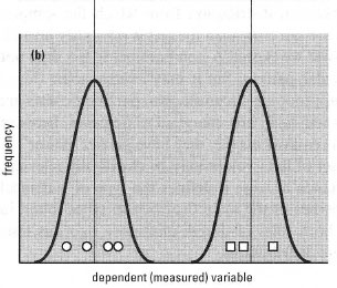Fig. 41.1 Two explanations for the difference between two means. In case (a) the two samples happen by chance to have come from opposite ends of the same frequency distribution, i.e. there is no true difference between the samples. In case (b) the two samples come from different frequency distributions, i.e. there is a true difference between the samples. In both cases, the means of the two samples are the same

A statistical test will indicate the probabilities of these options. The NH states that the two groups come from the same population (i.e. the treatment effects are negligible in the context of random variation). To test this, you calculate a test statistic from the data, and compare it with tabulated critical values giving the probability of obtaining the observed or a more extreme result by chance (see Boxes 41.1 and 41.2 below). This probability is sometimes called the significance of the test.

Note that you must take into account the degrees of freedom (d.f.) when looking up critical values of most test statistics. The d.f. is related to the size(s) of the samples studied; formulae for calculating it depend on the test being used. Chemists normally use two-tailed tests, i.e. we have no certainty beforehand that the treatment will have a positive or negative effect compared with the control (in a one-tailed test we expect one particular treatment to be bigger than the other). Be sure to use critical values for the correct type of test.

By convention, the critical probability for rejecting the NH is 5% (i.e. P = 0.05). This means we reject the NH if the observed result would have come up less than 1 time in 20 by chance. If the modulus of the test statistic is less than the tabulated critical value for P = 0.05, then we accept the NH and the result is said to be 'not significant' (NS for short). If the modulus of the test statistic is greater than the tabulated value for P = 0.05, then we reject the NH in favour of the alternative hypothesis that the treatments had different effects and the result is 'statistically significant'.

Two types of error are possible when making a conclusion on the basis of a statistical test. The first occurs if you reject the NH when it is true and the second if you accept the NH when it is false. To limit the chance of the first type of error, choose a lower probability, e.g. P = 0.01, but note that the critical value of the test statistic increases when you do this and results in the probability of the second error increasing. The conventional significance levels given in statistical tables (usually 0.05, 0.01, 0.001) are arbitrary. Increasing use of statistical computer programs is likely to lead to the actual probability of obtaining the calculated value of the test statistic being quoted (e.g. P = 0.037).

Note that if the NH is rejected, this does not tell you which of many alternative hypotheses is true. Also, it is important to distinguish between statistical and practical significance: identifying a statistically significant difference between two samples does not mean that this will carry any chemical importance.