Descriptive statistics

The purpose of most practical work is to observe and measure a particular characteristic of a chemical system. However, it would be extremely rare if the same value was obtained every time the characteristic was measured, or with every experimental subject. More commonly, such measurements will show variability, due to measurement error and sampling variation. Such variability can be displayed as a frequency distribution (e.g. Fig. 37.3), where the y axis shows the number of times (frequency, f) each particular value of the measured variable (Y) has been obtained. Descriptive (or summary) statistics quantify aspects of the frequency distribution of a sample (Box 40.1). You can use them to condense a large data set, for presentation in figures or tables. An additional application of descriptive statistics is to provide estimates of the true values of the underlying frequency distribution of the population being sampled, allowing the significance and precision of the experimental observations to be assessed.

*Note: The appropriate descriptive statistics to choose will depend on both the type of data, Le. whether quantitative, ranked or qualitative and the nature of the underlying frequency distribution.

In many instances, the normal (Gaussian) distribution best describes the observed pattern, giving a symmetrical, bell-shaped frequency distribution for example; replicate measurements of a particular characteristic (e.g.
repeated measurements of the end-point in a titration).

Three important features of a frequency distribution that can be summarized by descriptive statistics are:

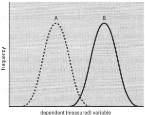
1. the sample's location, i.e. its position along a given dimension representing the dependent (measured) variable (Fig. 40.1);
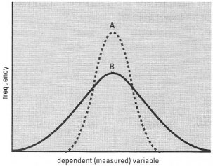
2. the dispersion of the data, i.e. how spread out the values are (Fig. 40.2);
3. the shape of the distribution, i.e. whether symmetrical, skewed, Ushaped, etc. (Fig. 40.3).

Fig. 40.1 Two distributions with different locations but the same dispersion. The data set labelled B could have been obtained by adding a constant to each datum in the data set labelled A.

Fig. 40.2 Two distributions with different dispersions but the same location. The data set labelled A covers a relatively narrow range of values of the dependent (measured) variable while that labelled B covers a wider range.

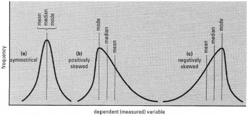Fig. 40.3 Symmetrical and skewed frequency distributions, showing relative positions of mean, median and mode.