Experimental design

There are two main multivariate optimization strategies: those based on sequential designs and those based on simultaneous designs.

Sequential design
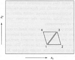
Sequential optimization is based on the one-at-a-time approach. The major limitation of this approach is that it assumes that no interaction effects occur between the variables. Unfortunately this is not always the case. A sequential design strategy involves carrying out a few experiments at a time and using the results of those experiments to determine the next experiment to be done. The best known of the sequential design approaches is called the simplex method. A simplex is essentially a geometric figure having a number of vertices equal to one more than the number of variables. For example, if we have two variables, the simplex is a triangle, three variables a tetrahedron, and so on.

Fig. 43.2 Simplex optimization.

Let us consider the case of two variables, x₁ and x₂. An algorithm describes the initial simplex to be performed (Fig. 43.2). By performing experiments 1-3, described by the initial simplex, and recording their responses, the next set of experiments can be described. If we obtain the lowest response for experiment 2, it can therefore be assumed that a higher response would be obtained in the opposite direction. By reflecting point 2, we can obtain point 4. By performing the experiment described by po int 4 we obtain its response, thereby perpetuating the simplex.

Four rules can be described for a simplex design:

1. A new simplex is formed by rejecting the point with the lowest response and replacing it with its mirror image across the line defined by the two remaining points.
2. If the new point in the simplex has the lowest response, return to the preceding simplex and create the new simplex by using instead the point with the second-lowest response.
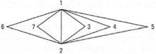
3. If a point is retained in three consecutive simplexes, then it can be assumed that an optimum has been reached. (Note: it may be that this optimum is not the true optimum, but that the simplex has been trapped at a false optimum. In this situation, it is necessary to start the simplex again, or use a modified simplex in which the step size is not fixed but variable, see Fig. 43.3.)
4. If a point is suggested by the simplex algorithm that is beyond the limit of the variables, i.e. it is beyond the safe working limits of an instrument, then the point is rejected and an artificially low response is assigned to it, and the simplex is continued with rules 1-3.

Fig. 43.3 Step-size simplex.

Simultaneous design
In a simultaneous approach the relationship between variables and results is studied as follows: carry out an appropriate design, apply a mathematical model to the design, and then apply a response surface method to the data. Appropriate designs might be based on factorial designs (full or fractional) or a central composite design. Response surface methods frequently rely on visualization of the data for interpretation.

Factorial design
In general terms, consider the case of two variables at two levels, e.g. a high value and a low value. This is termed a two-level design or a (full) 2^k factorial design, where k is the number of variables. Therefore we have 2² = 4 experiments to be done. Often the values of the variables are coded; this is done for convenience purposes only. In this example, high and low values will be coded as (+) and (−). Alternatively, it might be the case that the number of variables is three. In this situation we would have a 2³ factorial design, requiring eight experiments. An example of a two-level factorial design is shown in Box 43.1.

The limitation of the two-level factorial design approach is that no estimation of curvature can be determined. In order to take this into account the use of designs with at least three levels is required. Three-level designs are therefore often known as response surface designs. Probably the most important design in this context is the central composite design (CCD). Central composite designs consist of a full (or fractional) factorial design onto which is superimposed a star design. The number of experiments to be done (R) can be worked out as follows:

⇒ Equation [43.1]

R = 2k + 2k + n0

where k is the number of variables, and no is the number of experiments in the centre of the design.

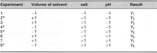
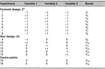
For a design with three variables we would require [2₃ + (2 × 3) + 1] = 15 experiments. In order to obtain repeatability information it is necessary to run an experiment several times. This is done by performing the centre point experiment twice. The total number of experiments would therefore be 16. The list of experiments is shown in Table 43.3 while Fig. 43.4 shows a diagrammatic representation of the CCD. The CCD is composed of a 3^k factorial design superimposed with a star design (+α, −α). In order to minimize systematic eror (bias) it is necessary randomize the experimental run order. This is shown in Table 43.4.

Table 43.2 Two-level factorial design

Table 43.3 Central composite design for three variables

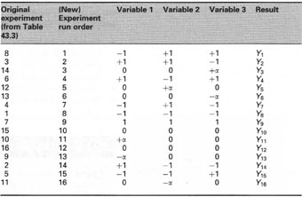Table 43.4 A typical randomized CCD